Have you heard about the Lattice Boltzmann Method? No?
…Or maybe you have, but you would like to know more details about it?
Then this article is for you!
My friend Nicolas Maquignon from France who is a PostDoctoral Researcher has massive experience in this area and he decided to write and share his knowledge about it with you all on this very blog.
I hope his article will bring new ideas to you!
Warning though… Nicolas made a big effort to keep the article simple, but it is still pretty advanced stuff…
so if you don’t understand fully, feel free to ask questions, comment or directly contact Nicolas (his contact is at the bottom of the page)
Here's a quick profile of Nicolas:
About the author:
Dr. Nicolas Maquignon
I am a PostDoctoral researcher who works in a French start-up located in Toulouse (south of France). My job is to develop physical models of explosions within a new FEA software using smoothed particle hydrodynamics methods (SPH)… and it’s really amazing!
1- Creating your own CFD solver with the Lattice Boltzmann Method, an alternate CFD model, from physics to computational physics
Before working on SPH, I developed equations and test cases simulation code in the field of the Lattice Boltzmann Method (LBM) for 5 years.
I used to study LBM equations for LNG (Liquefied Natural Gas) phase transition and scientific computing during my PhD and I could go through all this fascinating work thanks to a background in mechanical engineering.
I am always opened to discussions and debates in order to improve my understanding of numerical methods and also to help you to make your own idea... so if you have questions, don't hesitate!
Why the Lattice Boltzmann Method, you may ask... ?
The Lattice Boltzmann Method is a powerful method which is becoming famous and also a serious contender with traditional models used in CFD such as the finite element or finite volume methods…. and that’s why I decided to share all I know about it in this article today (Well, not ALL… obviously, but truly a lot)
LBM is a method which attracts many researchers and engineers, because it allows the incorporation of a lot of physics and because it has the advantage to be highly parallelisable.
Understand that LBM is very well suited for scientific CFD computing with Graphics Processing Units (GPU), which under certain circumstances can really accelerate the simulations.
LABS or POWERFLOW are examples of softwares that use LBM.
Using this method, many fluid behaviour become accessible, like turbulence, acoustics, phase transition, thermal fluids… It is used in the field of CFD modeling for transport ( ie train-flight), meteorology, porous media… And many other topics.
2- Boltzmann and links between microscopic and macroscopic scales
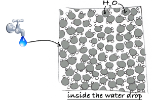
Do you know the difference between a fluid seen at the human scale (the macroscopic scale) and the same fluid seen at a molecular scale (the microscopic scale)?
A fluid at the macroscopic scale is a continuous material with certain properties (density, speed) and its behaviour can be described by the famous Navier-Stokes equations... at the microscopic scale, the fluid is seen as particles and thus quantities such as density or speed take a whole other meaning.
Most CFD programs are solvers that numerically integrate the macroscopic Navier-Stokes equations, using finite difference, finite volume, or finite element methodologies (plus a graphical interface maybe).
Never heard about Navier-Stokes Equations?
The Navier Stokes equations describe the temporal and spatial evolution of density, momentum and energy.
They can be solved in a Lagrangian or Eulerian framework, depending on the problem to study.
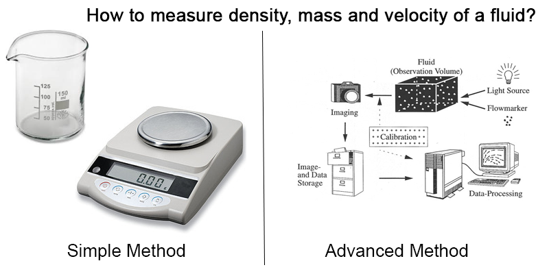
In this equation(s), density and velocity are continuous macroscopic variables, which implies that:
- They can be described by continuous functions
- We can measure them by means of appropriate instruments at the human scale
Ex: A simple balance and a dosing glass make it possible to measure a mass, a volume, and thus a density. More sophisticated methods as particle tracking velocimetry allow us to study the velocity field of a fluid. Pressure sensors can inform us about the pressure at some strategic points.
In a general way, at a macroscopic scale, it is mostly possible to numerically describe the behavior of a fluid, with more or less moderate computational resources, depending on the geometry and the conditions of turbulence and compressibility.
However, even if the events seem to happen in a globally coherent way on our scale, things are quite different when we try to study this same fluid on a microscopic scale, that is to say in a dimension where one can discern its particles, and where the apparent continuity on our scale is broken.
...but why the heck should I care about the microscopic scale and the fluid's molecules?
Indeed, why not staying with the standard macroscopic methods developed dozens of years before that until now seemed to suffice?
First, a fluid seen at its microscopic scale IS an ensemble of molecules which have an unexpected behavior (and unpredictable behaviour)... we can't just ignore that!
Second, establishing links between micro an macro scales improves our understanding of the fluid behaviour, and thus we may become able to use this knowledge to improve current known methods.
If you think about it, many of the scientific and engineering breakthrough of the last century have been due to some scientists such as Einstein who have been willing to look closer at the real physical behaviour ...
If scientists weren't willing to do that, we would still probably believe that the earth is flat... ;-)
The LBM method is a very promising CFD model, which will play an important role in the next following years in the field of CFD (and It also is a very interesting topic for those interested in theoretical and applied physics...)
Understanding the LBM can also open the gates to a deeper understanding of the calculations done by the solver of your FEA software.
Moreover, I actually encourage you to develop your own CFD code, using any known method...
Never just trust blindly softwares made by others (Why? Read this article from Cyprien to understand)…you will truly learn a lot by writing your own code.
Now... What are the big problems with the microscopic scale?
On this microscopic scale, certain notions which are familiar to us disappear...
Just think about it:
- How can you define a density, while a large vacuum surrounds the molecules of the fluid ?
- How do you define a velocity, while in an infinitesimal volume, the particles move in a disordered way and in all directions ?
- And...what is the link between the movements of particles and the observable properties of a fluid?
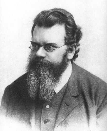
Those are the questions the brilliant physicist Ludwig Boltzmann [1844-1906] tried to answer.
He is the one who established first all the links and equations that lead to the Lattice Boltzmann Method.
That's what we will talk about next.
3- Case of a gas at steady state and zero velocity
Consider the case of a volume of air at rest in a room, without apparent movement, and static.
From our human point of view, this volume of air is inert and in the absence of thermal or mechanical disturbances from the external environment, this volume of air can remain in this state for a very long time… Let’s now zoom in on an infinitesimal portion of this volume of air.
What do we observe? Well, we observe everything except a static state ;-)
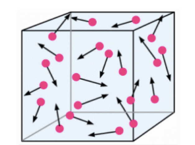
The particles are in motion relative to the reference frame of the room, and this in a completely disordered and completely random manner, at least in appearance...but appearances are often misleading …
In this apparent particle chaos actually hides information about the macroscopic properties of our fluid.
For the density of our volume of air, this is fairly easy to understand how to calculate it...
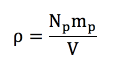
Because for a sufficiently large volume, defining a density actually means counting the number of particles:
mp is the mass of a particle and Np is the number of particles. The volume V corresponds simply to the volume of the room.
Here, shocks between particles are not taken into account. They are in any other case considered as hard, elastic and have no effect on the mass of the particles. Indeed, within the limit of Newtonian classical physics, the mass is preserved during collisions of particles.
Now ... how can we explain the velocity in a microscopic scale where velocities are so high and disordered that we see no global movement of the fluid at the macroscopic level?
4- A fundamental statement : Isotropy
First, we need to assume that the velocity vector of a particle can point in any direction. This statement seems quite obvious, as there isn’t any reason why an entity could not move into a certain direction.
This also means that there is no priviledged direction for the movement of a particle belonging to a fluid at rest. This is due to the fact that our geometrical space has the same properties in any direction, in other words it is isotropic. This property is responsible for the fact that the speed vector sum of the particles is zero.
This zero velocity vector sum is the speed we measure at the human scale, which explains why for a fluid at rest, we measure a zero velocity though a lot of disorder is present at the microscopic scale.
To summarise simply:
Isotropy = Same probability a particle moves to any direction = macroscopic velocity is zero
To demonstrate that, we need to do a bit of Maths ;-)
You can skip to the next section without much consequences if you’re not willing to go into some further mathematical details about it...
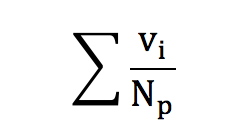
This property of isotropy is going to allow us to use a bit of math, to show that the vector sum of the particle velocities is zero. Let us assume an ensemble of particles « i » that have an individual speed norm and direction.
The speed vector sum V of this ensemble of particle can be written using Einstein summation convention :
In order to organise our algebraic development, we need to postulate that within a small range of speed norm [v-dv ;v+dv], every direction « k » is represented by a particle « j » owning the speed vj = v :
Thus, the analysis can be decomposed into a large number a small ranges [v-dv ;v+dv], correspondind to the spreading of speed magnitude. The calculations that are true for a certain speed range is also true for another speed range. The calculation can be simplified into :
Or with some simplified expression :
We have to suppose that a very large number of particles are present in our volume of study, in order to keep our approximations close to the continuum limit. This means that any direction or angle can be represented in a equi-probable proportion. This also means that for any a in [-1;1] :
Under the hypothesis that a very large number of particles are present, we could assume that the ensemble of particles behaves « almost » as in the continuum limit, and that the interval of vxk's is « dense ». Thus, we could make some strong assumption that we could arrange our sum of speed vector such as :
Thus, the vxk’s or vyk’s can be represented through an equi-probability distribution function on the [-1 ;1] interval. In the interval [-1 ;1], this distribution is simply :
Calculating the a mean value for vx, we have :
Calculating E(vx) we find E(vx)=0. This corresponds to the mean value of the vxk’s. Keeping in mind that :
So...that's it, we just demonstrated that the vector sum of particle velocities is 0 !
Though the vector sum is zero, this doesn’t mean that the mean speed magnitude value is also zero. The average speed is :
And the mean kinetic energy is :
We are now going to have a look at this kinetic energy and explain how it is related to temperature.
5- Air at 20°C and average kinetic energy
As I have just mentioned, though their directions are really disordered, the particles have a certain average magnitude velocity, which is non-zero.
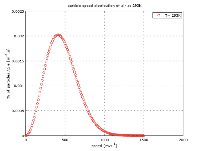
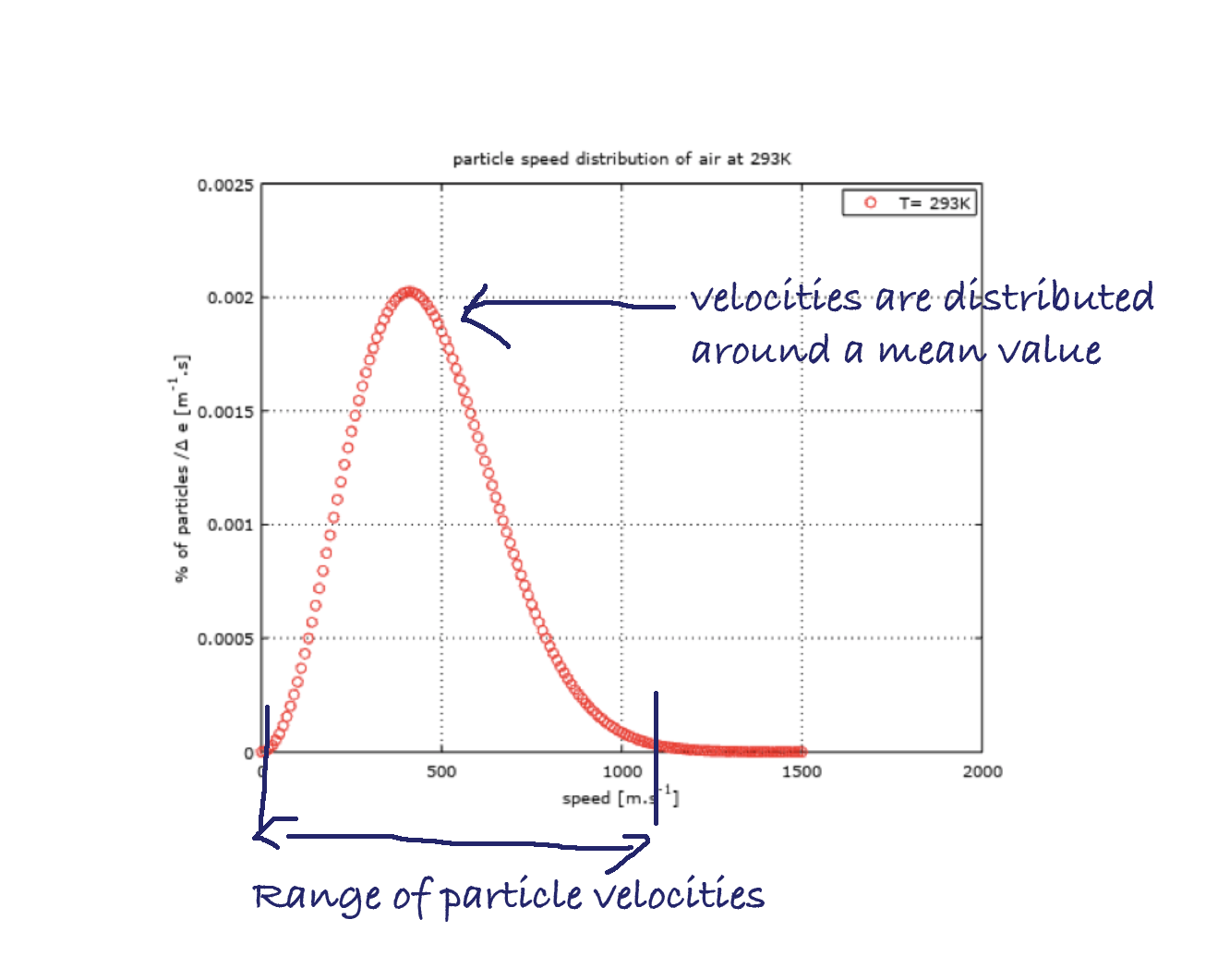
This speed magnitude is around 400 m/s for air at a temperature of 20°C, as shown in the following figure showing speed distribution on a red curve.
I ploted this curve with Octave (GNU) to show the distribution of speed magnitude within a volume of air at rest at ambiant temperature. X axis reprensents a speed interval, as Y axis corresponds to a percentage of particles within a certain range of speed.
If the distribution function is called f(x), we can calculate the probability for a particle to own a certain velocity magnitude within a range [a ;b] :
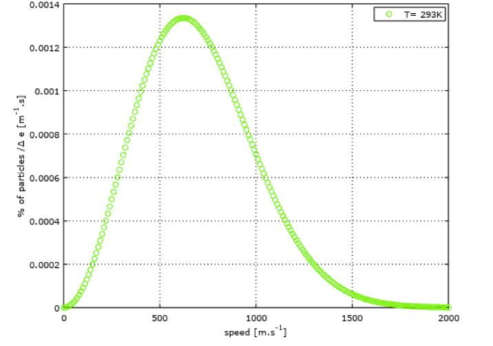
Note that it was here necessary to introduce the notion of temperature when fixing an average velocity value of the particles. This is because the temperature is related to the velocity of the particles. On the following figure (green curve), I ploted the velocity distribution for air at 400°C. We can observe that the mean velocity is now around 600 m/s and that the distribution range is widened, compared to air at 20°C.
Knowing about this particular distribution speed leads us to the distribution of energy in the fluid.
First, we need to introduce the notion of kinetic energy. Kinetic energy is the energy that something have due to its mass and its speed.
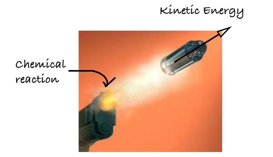
Taking the example of a bullet going out of a rifle, it is not beyond imagination that this bullet has a certain (large) energy, regarding all the trouble it could cause when it encounters an obstacle. The energy of the bullet comes from the chemical energy that was embeded in the gun-powder that has been converted into speed for the bullet at the moment of detonation.
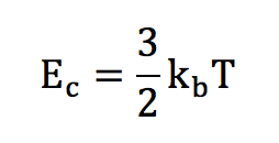
This « speed » energy is called kinetic energy. Boltzmann has established that there is in fact a link between the temperature and the kinetic energy of the particles, which is a function of the square of the velocity. Boltzmann tells us that for a monoatomic gas :
In this expression, the constant kb has appeared. This is a fundamental constant, called the Boltzmann’s constant.
The kinetic energy Ec that we get is in fact called the internal microscopic energy, as it contains the energy of the particles. If you try using this formula with some Argon, you’ll find a mean speed of 427 m/s.
6-Particule Position & Particle Velocity - Maxwell Distribution
The organization of particle velocities in disordered directions but with a fixed average magnitude, for a fixed temperature, can be further analyzed.
The mean energy may be fixed but nevertheless all the particles of an isothermal gas don't necessarily have the same kinetic energy.
In reality the velocities are distributed around a mean value, according to a certain organization. This is what we actually see in the previous red and green plots about speed magnitude distribution within a fluid at rest. This shows that the particles have a range of velocity magnitudes, distributed around a mean value which is located at the absciss of the maximum of the curve.
It is a priori not simple to find a probability law for a particle to have a certain velocity magnitude. However, for speed directions, the isotropy hypothesis, which leads to equiprobability of all directions, seems to hold, as we’ve just seen before.
To deal with the problem of speed magnitude distribution, we could postulate that a particle can have any kinetic energy, as long as the mean kinetic energy of the set of particles allows us to reconstruct a physically coherent macroscopic temperature, when summing over all the particles.
Only a fine observation of the properties of the particles, if it was possible, would teach us about the standard deviation around this mean kinetic energy (Appart from the averaged kinetic energy, the other statistical moments are also related to the macroscopic temperature).
Though, assuming that a particle can have any speed around an average value does not give us a precise idea about the distribution of velocities.
If we consider that each particle individually possesses a velocity according to an individually indeterminate probability law, the central limit theorem teaches us that for a large number of particles, the distribution law to be globally applied is the Gaussian normal law. Thus, the distribution of the speed magnitudes is done according to the normal law that follows :
This distribution law is the Maxwell equilibrium distribution, valid for a perfect gas.
The constant Rs is the specific gas constant, T is the temperature, e is the microscopic velocity of particles and u is the macroscopic velocity.
I used this formula to plot the red and green speed distribution curves, with u=0 for a fluid at rest.
For a perfect gas, the internal energy of the system is summed up in microscopic kinetic energy, because the potential inter-particle energy is considered as zero. A perfect gas is sufficiently dense for collisions to take place quite consistently.
7- Out-of-equilibrium distribution function and evolution
7-a-Phase space
The notion of "phase space" is an elementary concept that needs to be understood in the field of Lattice Boltzmann methods.
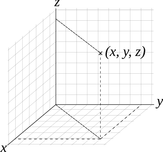
First, you surely have heard about the usual geometric space, which is modeled with three coordinates (x,y,z) in the Cartesian framework.
Cartesian space (source)
This space isn’t sufficient when we come to the description of particles, because we’ve seen how important the speed of the particles is. Indeed, the macroscopic properties does not only depend on spatial distrbution of particles, but it also depends on the speed distribution.
If we are to study the variations of these spatial and velocity distributions through time, we need to include the time in our coordinates.
The phase space corresponds to the gathering of geometric and velocity spaces.
7-b-Phase space distribution function
At equilibrium, the knowledge of the microscopic properties of air, or more generally of a perfect gas, is now accessible to us, thanks to the Maxwell equilibrium distribution that we have introduced earlier in the article.
However, the study of a fluid rarely summarizes to its equilibrium properties.
Limiting ourselves to equilibrium properties would forbid the study of many cases.
We must therefore open ourselves to the study of properties that are out of equilibrium by simply introducing the distribution of particles out of equilibrium into the phase space.
This distribution of particles in phase space can be defined by a function f:
It corresponds to the probability for a particle at a position [x] to possess a velocity [e] at a time [t].
From here you can skip to the next section if you’re not willing to go into some further mathematical details about it:
Following the principle of inertia, we know that the velocity distribution is preserved over time, in the absence of an external force field and in the absence of interparticle collisions.
In the absence of compression or relaxation, the spatial distribution remains essentially unchanged over time.
At low Mach and in the absence of collision, the differential of f is conserved. We can thus deduce the following equality:
The transport expression of f can then be obtained with a Taylor development:
In absence of external forces:
In the case of collisions, this equality must be modified by taking into account the variations of the probability distribution in the phase space. This factor will be called a collision operator, and we will not deal with its complex expression in detail.
We’ve just written here the Lattice Boltzman Equation (LBE).The collision operator can nevertheless be seen as a rate of variation, corresponding to a relaxation towards the equilibrium distribution. Thus, a reasonable approximation of this collision factor can be established :
This collision operator is know in the LBM community as the "BGK" collision operator or « Bhatnagar-Gross-Krook ».
8- Lattice and discrete form - advection/collision
Having now a transport equation, a discretization can be envisaged, in order to achieve a numerical integration.
In this article, we will not go into the mathematical detail of this discretization, because it is tedious and is not really essential for an elementary understanding of the LBM. Interested readers can refer to articles in the scientific literature (you can contact me if you’re interested).
It is important to understand that the space to be discretized is not a classical four-dimensional space. Indeed, since the distribution function is defined as a function of position, speed and time, it is not possible to use a single spatial mesh on which time iterations are to be calculated. The mesh must correspond to a whole phase space discretisation.
This means that the mesh must include geometrical nodes, but also « speed nodes ». Thus, one can imagine the use of a spatial mesh, in which a set of discrete velocities are represented.
This adds a constraint on our spatial mesh, which can not be realized in a completely free way because of the presence of speeds.
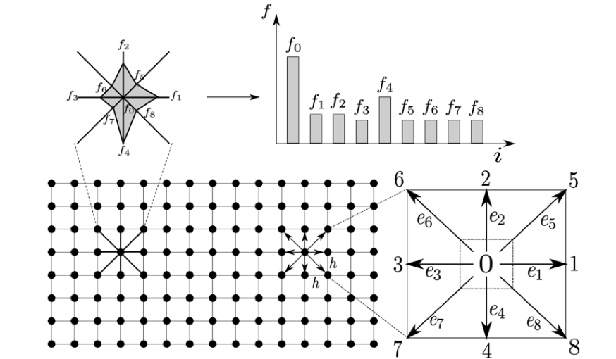
In the same way that a finite number of discrete spatial nodes can discretise the geometry of the problem we want to solve, we must define a set of discrete velocities representative of the set of velocities a particle could take. In practice and for 2D cases with little complexity, a set of 9 speeds are sufficiently representative.
Indeed, 9 speeds provide sufficient isotropy to the model and it is sufficient for weakly compressible fluid applications.
In a Cartesian mesh, these velocities are taken such that a particle present on a node can remain on this node, or else go to one of the 8 nodes that are located in its direct neighborhood.
2D problem is discretized with the Lattice Boltzmann framework (Source)
This case is called the D2Q9 lattice: that means two spatial dimensions and nine discrete velocities. Other types of LBM networks can be established, in 2D and 3D. For LBM lattices, the DnQm denomination is usually used. A DnQm Lattice means that the lattice has n spatial dimensions and m discrete speeds.
The black dots represent spatial nodes that are occupied by particles. A site does not contain only one particle but a certain number that depends on the local density.
In a time step, a particle can only move to its nearest neighbors sites, with one of the discrete speeds that are here noted ei, with i from 0 to 8. We all together have 9 discrete velocities.
The fi’s represent the number of particles that move with a discrete speed ei. For a site containing N particles, fi*N particles move with a speed ei.
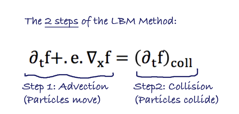
Once the ensemble particles have moved (advection) the one of the neighbouring site, they will collide with other ensemble of particles that arrive on the same site at the same time.
We have here identified the two fundamental steps of the LBM algorithm : advection and collision. And of course, the collision can be calculated with the collision operator that we have introduced earlier. The advection corresponds to the left had side of the LBM, and the collision corresponds to the right hand side of the LBE depicted before.
9- Discrete Equation and Algorithm
Since the different notions relating to the discretization of the phase space are now posed, it remains to describe the discrete form of the Boltzmann equation on a lattice of type DnQm.
Directly, this equation takes the following form, for a direction i of discrete speed:
The left term is a term of transport or advection. A Taylor development can also highlight a form of Lagrangian transport. The term on the right is the collision operator, it corresponds to the rule that applies when two particles arrive at the same time on a geometric node.
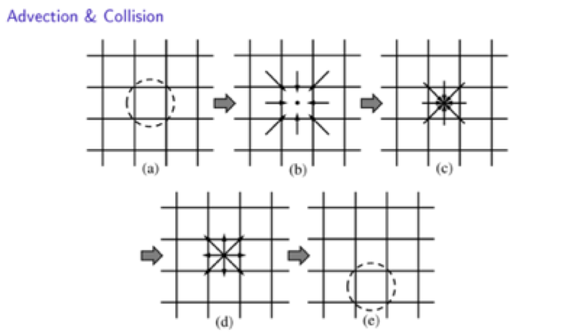
Based on this Boltzmann equation on lattice - LBM - an algorithm can be defined.
This is illustrated in the previous figure, and the steps are:
- Selection of a site
- Advection of incoming particles from direct neighbourhood.
- Collision of the new set of particles that have just been advected.
- Post-collision rearrangement
- Next site selection
10- An example : the pressure pulse
For this example, I wrote a D3Q19 LBM solver using C language under some ubuntu environment (If you’re interested in getting the code, please contact me. )
The pressure pulse is an elementary benchmark you can use to validate an implementation for some cases.
Here, the topic of pressure pulse is rather in the field of acoustics, as it can model very small pressure variations. This doesn’t mean that all we’ve seen before is only available for acoustics!
All the tools we’ve seen are quite powerful, and it can in general solve cases for low Mach laminar fluids. Some small modifications can bring the model up to soft turbulence modeling. Of course, if you’re interested in more complex flow, you should bring some further modifications.
The initialisation of the case is quite straightforward : A pressure peak is initialised at the center of the domain. I mean the density is initialised in a uniform manner, except at the center where a small pressure shoot is added to the average density, as it can be seen on the first 2D view of the following figures. The whole domain is initiaded with zero velocity. The boundary conditions are periodic. The mesh is cartesian and uniform has depicted earliear.
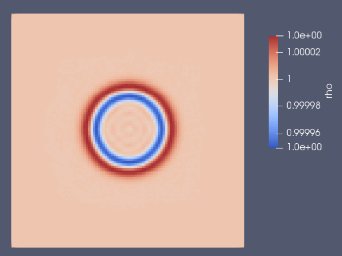
The spatial step is of 1.0 cm, and the time step is of 17.28 e-6 s. The speed of sound is set at 334 m/s, which is the speed of sound of air at 20°C. The physical simulation time is of 0.5 ms. I ploted illustration using Paraview (GNU) in order to depict initialisation and results :
Initialisation of density field :
Density field after 0.5 ms of physical simulation time :
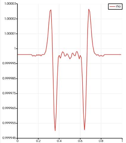
We can observe that the initial density peak (linear to pressure) spreads to a slighly higher pressure wave, followed by a rarefaction wave : this is typical of that kind of test case, and it validates our implementation in a qualitative manner. The two following plots show a radial profile of the density (there is a spherical symmetry), at the initialisation and after the 0.5 ms of physical time:
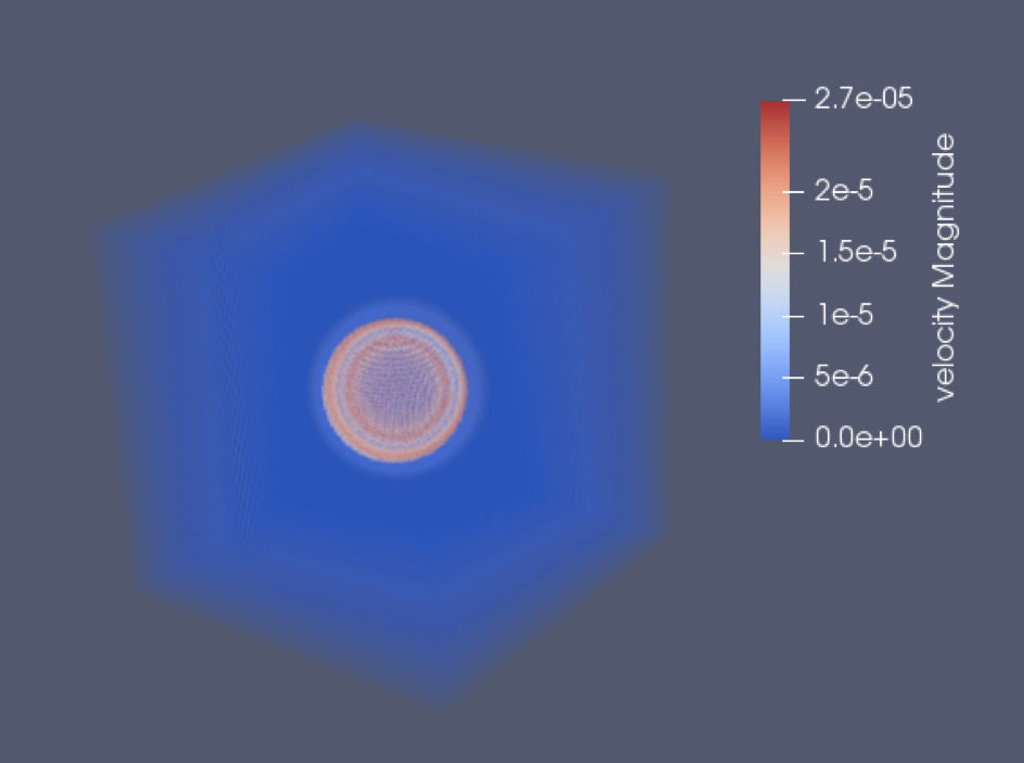
We can observe the higher pressure peak followed by the rarefaction peak. And if we measure the distance that the high pressure speed has done during the simulation, and we divide it by the physical time, we find 334 m/s… Which is indeed the speed of sound that we set as parameter. This validates the code in a quantitative manner, though a comparison to analytical solution would still be interesting (for the readers who would like to go further). The two last figures show density and velocity fields at the end of the simulation in 3D.
Author :
Nicolas Maquignon. Ph.D.
Postdoctoral Researcher @ Impetus AFEA France
Contact: nicolas.maquignon@gmail.com
———–
That’s all basically for this article… and that's a LOT of knowledge to unpack ;-)
Take all the time you need to read and if you want to share your ideas, please just write what you think in the comments and let me know
Thank you so much for reading, I hope you learned a lot!
–Cyprien















nice post!!! really interesting and useful….
Greetings from Mexico!
Thanks ! Fell free to ask any question on this topic !
for the reference values of density, speed, and speed of sound. here which the speed of sound is used? I mean the speed of sound in the air, or water or the liquid under consideration?
Another question is shall have a D2Q9 code written in Fortran 90 to compare with mine whether it is right or not.
Kind Regards
It was a great article indeed but there are a lot of information that could not be understood by me. If I would ask you the more basics of this idea including the basics of mathematical formulas, how to solve them and basics of programming from where a beginner may start to work on LBM. Kindly guide me in this regard.
Great work!! Thanks for sharing your knowledge on LBM.
Looking forward for more posts from you.
Thanks for appreciating this post !
Excellent take on LBM. Looking forward for more such articles and if possible a graphic tutorial on how to implement LBM.
Thanks.
thx Rupak !
Really nice post!! thank
Thx Magaly !
That is one very good article on LBM.
I however want to know more about SRT and MRT.
What difference it brings when we implement MRT?
I would formally mail you regarding all my doubts.
Hi Vaibhav, thx for your interest.
SRT uses only one relaxation parameter, and MRT uses as many relaxation parameters as the number of discrete speeds (ie. 9 relaxation parameters for D2Q9). With MRT, the collision operator is calculated in the space of moments. So every moment relaxes to a different rate. The MRT takes it longer to implement, and computational time is a bit increased. also, it requires more memory. But there is a lot to say about MRT! if you have further question don’t hesitate to mail me.
Très sympa! ça m’aide vraiment beaucoup!
Super! si vous avez besoin de précisions sur le sujet, n’hésitez pas!
Est-ce que tu pense que ç’est intéressant d’utiliser LBM sur les grandes échelles?
Je dirais que ça dépend du type de problème de grande échelle… Clairement, le côté très parallélisable du modèle est son atout essentiel. Alors oui sur un problème grande échelle avec de grandes quantités de données cela peut avoir un intérêt. Après de là à dire que ça sera forcément plus performant et plus précis qu’un modèle plus classique…
you made it available all at a single place , very well crafted article. thanks bro.
greetings from INDIA .
Amazing article. I’m fairly new to LBM I was wondering if I could get some advice. Currently I use MATLAB to write LBM simulations. Is there any disadvantage to using MATLAB ? I see that most people tend to write their codes in C or C++. Thanks in advance!
The problem with MATLAB is that it is quite slow… when in such numerical scheme algorithms you really need speed of computation. That’s why most FEA software and serious engineering tools (as well as game graphical engines ;-) ) are generally written in C or C++. It’s more complex to write, but it’s much faster.
I liked reading this article. It seemed to clean up my chaos a bit :D
Thank you!
Ten years ago, I tried to write that public LBM D2Q9 pseudo-code in 386 assembler and it worked fine… until the simulation ‘just fucked up’ ;-) It’s like, no matter how low I put the density in the cells, after some time, it rises, becomes super turbulent and then, the simulation gets ‘spreading cancer’, eating up all floating-point numbers to end up with ‘not a number’. I tried to circumvent this by using a ‘dynamic compressor’, but it made the image become unsharp… although over time, the results still seemed to look natural.
Now I have to correct it, to be able to simulate the soundfront inside my diy-loudspeakers. I’m assuming that all partial waves have to leave the bass-port together as one, to avoid harmonics (causing dips and peaks) and to give good sound-pressure.
You seems to have a very interesting experience Alexandre. I have to say that programming such code in Assembleur must be quite a Challenge ;-) Maybe you could post the code (If you can find it back) and see if someone who read the article gets a solution…
Thanks for a great article! Best of luck and keep your enthusiasm for helping others to understand things that at faculty was hard to understand!
Excelent compendium. Shall be part of book to be referred to.
This is a very good LBM introduction for beginners.
3-4 years ago I started to use grid-based CFD (OpenFOAM) and DEM (LAMMPS) to study the interaction between free-surface flow and irregular-shaped particles. On the side of modelling particle dynamics, there were no big issues as DEM is mesh-less. However, when it comes to fully resolving the interaction between fluid and semi-submerged solid particles, there are 3 types of interface within one CFD cell: namely gas-solid, liquid-solid, and gas-liquid-solid at the free surface. I had some troubles to calculate the pressure gradient and viscous forces acting on the solid particles, as it needs to located the exact cells on the fluid-solid interface, and the associated quantities such as porosity, velocity and pressure, etc. As a fully functioned CFD code (OpenFOAM), the source code is massive and complex: it is hard to get down to the low-level. and had a feeling that you have no full control on what is happening in you modified solvers.
After digging into the 2 alternatives to conventional CFD, aka SPH and Lattice Boltzmann recently, I found out it is much easier to write a CFD code with SPH or LBM compared to the grid-based CFD, because you don’t have to deal with the mesh! If I would have started my work on LBM or SPH, a lot of pain might have been avoided.
Currently I finished writing a 2D DEM (Discrete Element Method) code to simulate rigid body dynamics with arbitrary particle shapes. For the first time I felt having the full control over what is exactly happening behind the simulation. And more importantly, I can add some convenient/necessary features to the code much easier than to a fully-functioned open-source software, because you will have to spend a of time (months) to understand the original codes in the first place.
At the moment I am implementing a 2D SPH code, because it is pretty much the same as discrete element method, and most of my code can be re-used. It should not cost me a lot of time.
After reading this article, I thought I need to write a 2D LBM code, as it seems very promising and easier to implement, given the fact that it is based on uniform lattice, and incorporates some microscopic physics on the molecular level. I have some questions to ask for the OP: 1) Is it relatively easier to model free-surface flow (like water waves) compared to grid-based CFD? and what technique is most popular (like VOF); 2) Is immersed boundary method (IBM) already well established in LBM for fluid-moving bodies interaction (FSI)?
Best regards
Hi David, thanks for your interest.
LBM with VOF is popular for solving free surface flows – you can have a look at the thesis work of Niels Turey. IBM is also well established as moving boundaries. It’s implemented in commercial softwares and is present in the LBM litterature.
Hi Nicolas, great article and thanks for taking the time to write it out in such detail.
Next month I will be attempting to use a commercial LBM code (XFlow) to model unsteady multiphase (solid particles entrained in a viscous liquid) flow for industrial purposes.
I am very comfortable with advanced FEA for solid mechanics, but don’t have as much experience with CFD so it’s likely to be a challenging project.
Do you have any resources that might help me with the practical implementation of LBM? If you are able to offer me any advice on how to avoid common mistakes then I’d really appreciate it.
Best regards
Hi Nicolas,
Good article for beginners. I have few questions.
1. Is LBM lagrangian, Eulerian or Eulerian-Lagrangian method ?
2. In any domain (with grid), does fluid particles flushed out of the domain and replaced by new particles?
Best Regards
Hi,
1. I think LBM is a Lagrangian method, looking at some derivation step in which you use the material derivative as if it were a partial derivative, we could discuss it if you’re interested. Though all discrete speeds are imposed, and no particles “leak” the domain.
2. In boundary conditions, it could be seen as you mention, particles that flush out of the domain are immediatly replaced so no particle are missing.
I feel it is Eulerian or Hybrid. Take an aerodynamics simulation with virtual wind tunnel, we are collecting information at distribution functions from fluid particles. Here for a lattice, distribution functions are fixed but particles are passing through for each time step.
Also we are not showing interest to trace the particles which is nothing but lagrangian tracking.
I believe LBM is capable of solving both the ways and hybrid(correct me).
https://tel.archives-ouvertes.fr/tel-01522791/document
– look at equation (19) & (20) p. 139, a material derivative is used for integration.
This is what makes me believe it is Lagrangian, from a mathematical point of view.
But I agree on the fact that any simulation with LBM looks Eulerian.
but I admit I am not certain about this. this also is a question I’ve been thinking about for a long time.
It is interpretation. We can represent the equation in Lagrangian or Eulerian based on the point of interest.
Correct me if I’m understanding in wrong way
Hello
My name is Shim dae shick.
And I am working as CFD engineer in Korea.
I have worked as CFD engineer in korea company for 7years.
But I have little knowledge about CFD code. Because my master degree is MEMS
and my works focused on modeling, meshing ans consulting and other things.
After 7 years of engineering works, I determined to be a CFD code engineer and go to master / Ph.D course.
My interesting CFD field is LBM (lattice Boltzmann method).
I wish to know the university (CFD) in germany and Canada which are famous for LBM CFD coding
thanks
Hi Nicolas,
thank you for the intro!
I wonder, if LBM (or SPH) are used for combustion modelling (non-premixed) and conjugate heat transfer!? And what would be the advantages of SPH over LBM for such cases?
Thanks in advance!
Best Regards
bonne méthode !
j’ai une question est ce que ça serait mieux de travailler avec la LBM au lieu de RANS pour des études thermo-aéroliques
LBM DNS, sûrement pas. Il te faut une modélisation de la turbulence, sinon les choses seront incalculables. Peut-être que ça peut marcher en LES, mais il y a aussi des possibilités d’adaptation de RANS
Hello Everyone
I work on the numerical simulation of the natural convection in a cylindrical cavity by lattice Boltzman method and I try to to implement the cylindrical boundary conditions in motion in a FORTRAN or C++ code, if you can suggest to me a basic codes , I will be very grateful
thank you
email: farkachyounes@gmail.com
I suggest thermal flux bc and bounce back for the cylinder, for example. The problem of natural convection from cylinder is well known, you can find many references on the topic.
thank you
do you mean ‘references’ in this website ?
it’s a super clear introduction of lbm, I appreciate it!
I am using LBM doing acoustic and elastic wave modeling for seismic application.
I am a little confused about the source term here. so the source is added to the density not the distribution functions?
can you show a little bit of code to explicit how you load source?
Thanks!
To be clear, acoustic source term is a complicated topic. Here, the source is kinda mocked using particular ic on density. There’s no source term added,in other words. I suggest to add a ponctual normal density distribution at fixed frequency and density so to enforce pressure fluctuation. But this is not mass conservative
Thanks Nicolos, its a very interesting and most effective article for the LBM beginners. Greetings from INDIA!
being a beginner in this field, I have interested in getting codes for some benchmark problems like, Lid driven cavity,Backward facing step , flow over circular and square cylinder. and how to get equilibrium distribution function for collision.
Thanks in advance.
Hello dear Nicolas ,
I am Evani Porto from Brazil.
I have read your article. It helped me to clarify some doubts. Thank you!
But I still have some problems im my simulation. I would be very glad if you could say something to help me.. :D
My algorithim is calculating the drag force “Cd” around cylinder accordingly to some results available in literarature, but the vorticity is not happening…. I am running the programing by more than 10.000 timesteps and the vortices does not appear….
I am using BGK D2Q9 with bounce-back condition, a cylinder with 40 nodes, Reynolds = 100 and a grid with 500×250 .
Is there any critical point for the vorticity appeareance ?
What coulde be a crucial step to not miss on the simulation?
Thank you very much ;;
Hi ! Nice question – actualy your Reynolds number is a bit low for laminar vortices to appear. Though the limit is of 90 if I remember correctly. Your numerical scheme is a bit too dissipative. I think BGK don’t fully capture the transition at which laminar vortices come. Try increase your Reynolds by decreasing a bit your relaxation parameter. Keep me updated !
Hi Dr Nicolas Maquignon..
I wrote you an email if you’re free to respond. Thanks
Please resend, I might have lost it.
Very helpful!
This post does save me from all the major confusions about LBM.
Thanks a lot!
Thanks. This is the propose of this article. I aim to make things understandable.
Thank you very much for your post!
I am a beginner at fluid dynamics and my interest is the aerodynamics.
May you recommend some articles about scale factor, Reynolds number for LBM?
As I know big body and small body with the same shapes will give different solutions. How does it works in LBM?
Oh, I didn’t notice
http://feaforall.com/implementation-lattice-boltzmann-method-lbm/
yep ! it’s all explained there !
Hi Dear! Can you tell me about the dependence of no. of body points while creating the geometry in excel? Does it affect the solution? I am solving flow past a square cylinder and I am using 100 points of square in excel to make it but as I vary the no. of points, it varies the solution. What is the reason?
the reason is simple, the more points you put, the more detail you get. and if you don’t adapt your relaxation parameter, increasing the number of points will make the Reynolds number vary.
I am sorry but how merely varying the number of interpolation points will change the Reynolds number? I am not using any relation of no. of points with the Reynolds number. Also is there anything related to MRT relaxation parameter with the Reynolds number? As in MRT, the last two moments usually named as s7 and s8 in the D2Q9 lattice model are taken as reciprocal of relaxation parameters. But we give the fixed tau value in input file before starting our simulation. Should we change that for variation in Reynolds number? Being more specific I want to simulate flow past a square cylinder at 2100 Reynolds number. What value of tau should be used for MRT and what grid? Looking forward for your kind reply.
Ahsan
yes, tau has to be recalculated if you use a different grid. for MRT, the relaxation parameter that corresponds to tau has to be changed, it is the most important parameter. others are fixed so to obtain the best possible stability, and one parameters is not important for non compressible problems.
What does it mean to be recalculated ? We give fixed value of tau say 0.51 or 0.505 before starting our simulation.
http://feaforall.com/implementation-lattice-boltzmann-method-lbm/
it’s all explained there
Hi everyone! Such a usefull article.
Im trying to learn LBM by my self (by arround two months nearly) and for sure I have a lot a doubts.
But the most relevants (im working in Pouseillie flow like my first simulation) are, if i consider a no incompresible flow why theres a “varation” in the densityt value? Also with the pressure gradient, how can I put it in initial condition and whats the correct way to do that? Like a force? Like boundary condition?
I apologyze if my questions are pretty simples.
Thanks ! Grettings from Chihuahua México!
(if someone have some book´s name o article of LBM examples could share me I´ll very very thankfull)
Hi Nicolas
Nice job…!!!
I just started my Ph.D. in Hydrogen Explosion Simulations.
I am trying to get an overview of the different methods in CFD simulations.
If you have any suggestions, please write me.
Regards
Javier
Nice article, I’m trying to learn about the Lattice Boltzmann method and of all the resources I could find this one is the easiest to understand.
I would like to suggest a small correction to section 6 though. The speed magnitudes of the particles in an ideal gas are not normally distributed. Rather, it is the velocity vectors that are normally distributed. The correct density for the Maxwell Boltzmann distribution is
f(u)=\sqrt(2 /pi ) u^2 .(R_s T)^{-3/2} .exp(-x^2 / (2R_s T) )
The set of 3D vectors which have magnitude u form the surface of a sphere, whose surface area is proportional to u^2, so the density for the normal distribution has to be multiplied by a factor of u^2 * (normalisation constant) to get the density of the Maxwell Boltzmann distribution.
Great tutorial. Thanks