[Full Tutorial] Linear Static FEA Simulation of a Wrench with Salome Meca

Hello guys. Cyprien here from FEAforall.

in this article, we’ll have a look at how to simulate a wrench into Salome Meca with Code_Aster and I’ll be using Aster Study to do this.

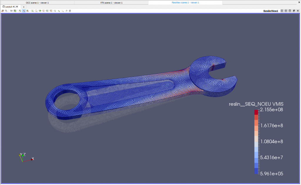
In this video I’ll really go into the details at how to get a very nice mesh, how to get some kind of transparency, how to animate all of this, how to apply a lot of filters and Paravis to extract the right mesh stress distribution.

What you will learn:

• How to Import CAD Geometry in Salome Meca
• How to Mesh is correctly (and refine the mesh afterwards) – How to prepare it for simulation
• How to create the Simulation Phase in Aster Study and Solve it with Code_Aster
• How to postprocess the results (including stress, deformation, animation, etc…)

Video Tutorial

After you watch the video, let me know what you think

If you like what I’m doing, please give it a ‘like” and subscribe to my channel and let me know if you have any comments.

You can download the model here

If something doesn’t work for you, if you have questions while you’re watching this video, please leave a comment on the video or on the blog. Let me know. And if I know the answer I’ll reply to you.

Step 1 – New Project Creation & CAD Import

So let’s start. I just opened a new window of Salome Meca.

I’m using the 8.3 version and there are some new versions released right now, I think, but I felt on this one was a bit more stable and less errors, so in case you get some errors with the latest version, you can switch back to this one.

I’m using the Windows version. So the Windows version isn’t officially supported by the team who is developing this Salome Meca, but it works rather well for simple static study. So that’s what I’ll use.

You can download Salome Meca for Windows here

Let’s start by creating a new document and opening the GEOM module in which I will load my CAD file (you can get it here)

Let’s go into the file and let’s import my STEP file:

I will have a dialog box telling me that there is a limit to a unit, which is embedded into the file and I can choose to ignore it or not. So it looks like it’s not very important but it’s actually pretty important because based on if you choose, “Yes,” the model will arrive in millimeter unit, but, “No,” it will be loaded in meta unit so your model will be a thousand times bigger. So I’ll choose “Yes,” and you see the model is very small here because it’s in millimeter unit.

You can zoom like that, and I’ll make sure that I chose the right choice. Never trust the model like that because if you just look at the diameter here you don’t really know. And sometimes you go over the whole analysis and you realize that the final result is wrong, you don’t know why, and that’s probably because of something like that.

let’s go into the “Inspection” Menu and there is a dimension bounding box feature that I can use to, basically, draw a bounding box around the model. And we see that the X-axis is comprised between -0.17 and 0.02.

And because the main unit I will use is meter (SI unit) when I do that, so if I think that I’m now in meter unit and this dimension is 0.17 meter, which is 117 millimeter… which is fine. It’s exactly what I want. So I’m okay. I’ll just close that.

Now I have to prepare for the next step. I have to think about what kind of boundary condition I’ll be assigning to this. So right now I extract the right surface groups that will be used to extract the mesh groups and to compute.

So what I’ll do is that I will fix the two faces on at head of the wrench and I will apply a pressure on the two faces at the top of the handle. So I need, basically, to extract those faces now.

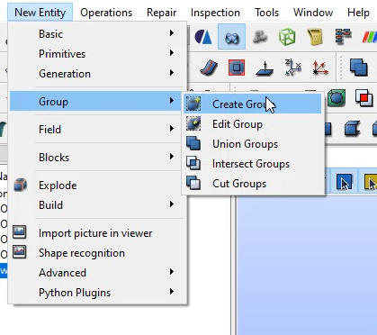
So let’s go into “New Entity> group”, “Create group”, and now I just have to select the right faces. So one face here. then “Next.” “Select” … Okay, let me just … Selected one. Make sure you select the right faces. Okay. So this will be the “Fixed faces.” “Apply.”

Now let’s choose the two other faces for the load group.

So sometimes the faces can be selected, so I found out that you have to rotate a little more like that, and I press “Shift” to select two faces at the same time. Okay. Now I got two faces and those will be pressure surface, so we can call it “Press-surf”, like that. Okay. So let’s just check that I selected the right faces. You see by default when I selected the groups everything else gets hidden in the object browser tree so you can reactivate that.

I’m just making sure that I have selected the right faces, which it seems to be good.

Step 2 – Preparing the Mesh

Okay, so now I’m okay with the geometry. This wasn’t very complex because the CAD is already ready, right?

Now we can go into the meshing step. Let’s go into “Smesh” module and let’s create a mesh set for that.

Click on “Create a mesh set”

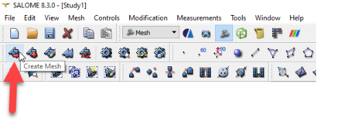
I’ll just use the simpler option for this because when the CAD is not very proper to make a hexahedron or some other type of special mesh.

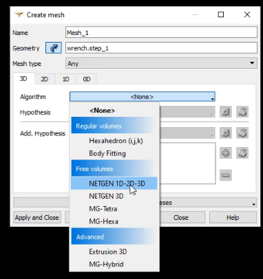
Click on “Algorithm” and choose: “NETGEN 1D-2D-3D.” This will be almost automatic. You won’t have to set up the 2D and 1D mesh algorithms, et cetera.

Then I have to assign some hypothesis parameters which will be used to define the mesh size:

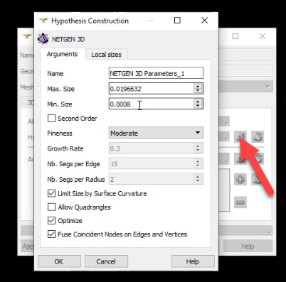
I’ll show you a bit later in the tutorial how to refine the size of the mesh. For the moment I’ll just go with a standard mesh just to see what I get.

Right click on your Mesh_1 instance in the object browser and click on “Compute” :

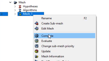
You will then obtain a mesh like this one (click on reset to resize the view):

This mesh is really coarse in some areas and fine in some others. I might have to refine it right now because this is first order elements so it doesn’t even follow the curvature of the CAD model:

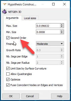
Let me show you the difference between first order and second order. “Second order” …

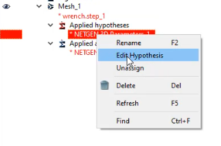
Let’s open the mesh and the hypothesis that you applied to which are shown in red. Click on “Edit” and you will be able to change the options used for meshing:

Select the “Second order” option and click on “OK”.

Sometimes you still have some nodes and you don’t want that because it might create problems when you remesh using those nodes. Right click on Mesh_1 and clear the mesh data totally.

And then I just “Re-mesh”. Let’s see if I get something better:

Now the elements go along the curvature. They are roughly the same size but they have now a node in the middle which allows for a better approximation of the curvature. We also see very clearly that those triangles are not any more just composed of one surface per element, they have some middle nodes which are making them into 2nd order triangles.

Let’s refine it a bit more. Just a bit more for this first try:

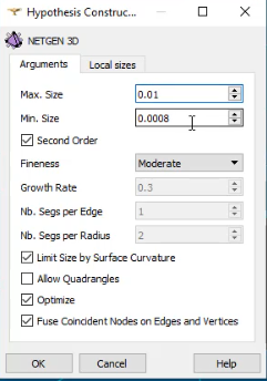
When you edit the hypothesis, there are a “Max size” and a “Min size.” The “Max Size” parameter controls mostly the size of the mesh in this case.

Let’s clear “Mesh data,” and “Re-mesh.” Now, I’ll just go with that and then I’ll refine later. That will be a good point to show you how, once you generate all the model, you can still come back to your mesh and refine it without having to change all your study.

Once I’m good with all of that, I will generate the mesh groups.

I created two geometry groups and I need to do the same, but for the mesh because what the Code_Aster solver reads is, ultimately, the mesh groups, not the geometry groups.

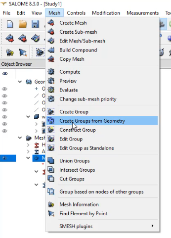
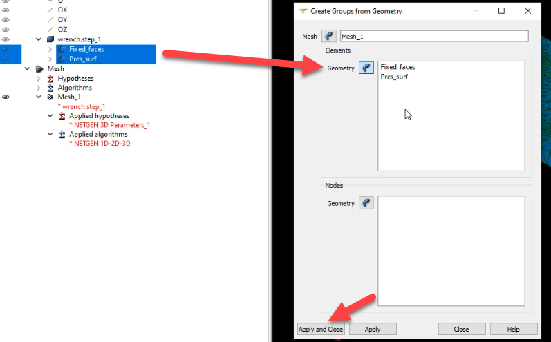
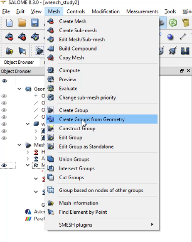
Go into the “Mesh” Tab and there is a very useful function called “Create groups from geometry.” This will allow you to select directly your geometry groups like this.

You press the little arrow here and this will appear here. “Apply,” and they will be created.

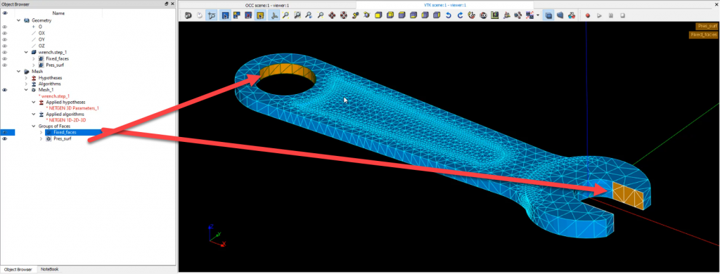
Let’s have a look. They are actually hidden by default so if you activate them you see that they appear in a different color, which allows to really see what are those mesh groups.

And now I am okay with that. Well, I mean, I’m not really okay because those mesh are really huge and I probably won’t get good results but that’s for the first try. Always start with something a bit coarse because it will be faster to compute and to correct your mistakes. If you take something very, very small from the beginning, and every time you try to iterate to try to correct your model, it takes a lot of time to calculate and then, basically, you lose a lot of time for nothing. If you’re model is coarse you can easily debug it.

Okay, so the mesh is done now.

Because I will use Aster Study, I don’t need to export the mesh. I can directly read it from Aster Study. But in case you would like to use Code_Aster solver without Aster Study, you could just export your mesh.

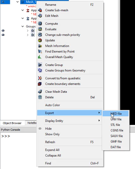
There is a function “Export into a Med file,” for example, and then read it again so you can have a separate mesh file. I don’t need to do that for this analysis because I will it be able to read it directly from the Aster Study case.

Step 3 – Setting up the Aster Study Analysis Case

Now let’s switch to Aster Study.

Let’s choose the “Stable version.” Now, let’s go and create a new stage for this simulation, and now that this stage is added all those options will be available for you.

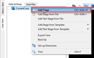
And, basically, to create this simulation I have to go in a certain order. And it’s more or less always the same thing for linear static analysis. So if you understand this process, you just have to follow it:

• Read the Mesh
• Create and assign the material model
• Define a Finite Element Model
• Define the Loads
• Define the Analysis Case
• Choose the additional outputs
• Select the result output file

The first step is always to read the mesh.

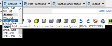
The names in the menu are a bit squeezed so it’s difficult to see what is written, but if you leave the mouse a certain moment on the menu item you’ll see the full name appearing in a tool-tip (The Linux version looks a bit better).

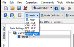
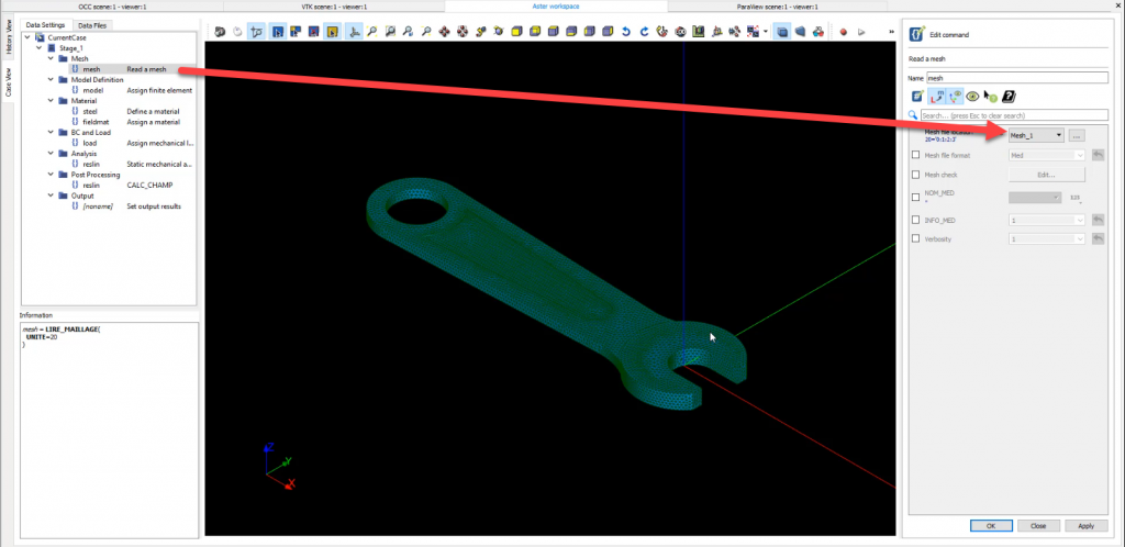
In the dialogue box which appears you just have to select your mesh. So if your mesh is in the S-mesh module, like I did, it will appear like that in the drop down menu. So you just have to click on the drop down. If this an external mesh that you have from another software or maybe you already exported it to met file, then you’ll have to click on the three dots and find your file in your computer.

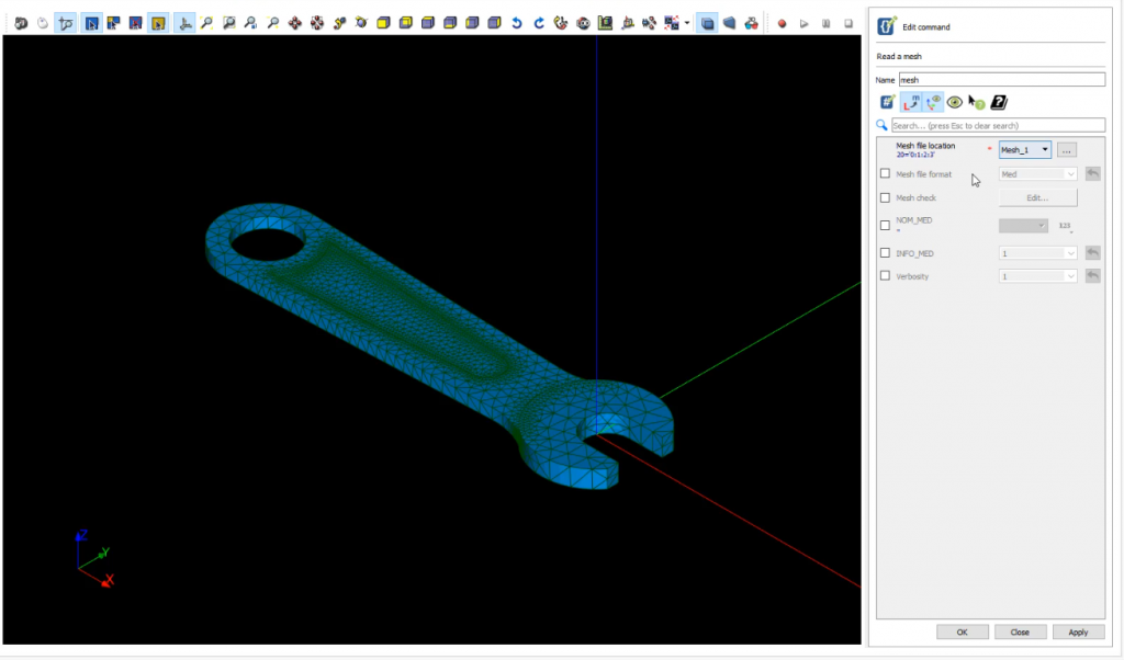
Okay. So now you see my mesh is imported so everything is fine. I don’t see the mesh groups but the mesh groups will be imported at the same time. So that should be fine.

Next step is to … It can be assign a “Finite element model” or it can be to “Create a material.” Let’s start by creating a material first and start with “Define the material.”

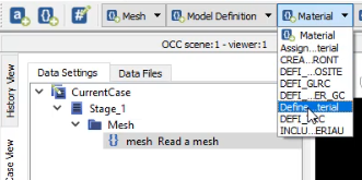
So I have to first create a certain material. So I just use “Steel material”. And you have to choose a type of model for the material. So you see you have a lot of models available, but just remember for linear material the simplest one is just “Linear isotropic elastic.” So just click on that.

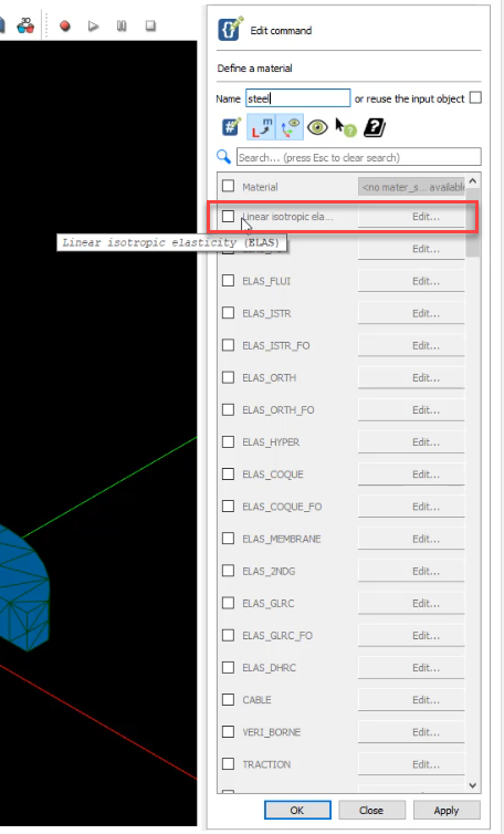
Then you have to input the Young’s Modulus and the Poisson’s ratio. One of the frequent mistake are to input the Young’s Modulus and the Poisson’s ratio here with wrong units.

So make sure that if you are working in meter unit, Young’s Modulus is also defined in Pa (N.m-2), not in mPa or in GPa. It should be in Pa.

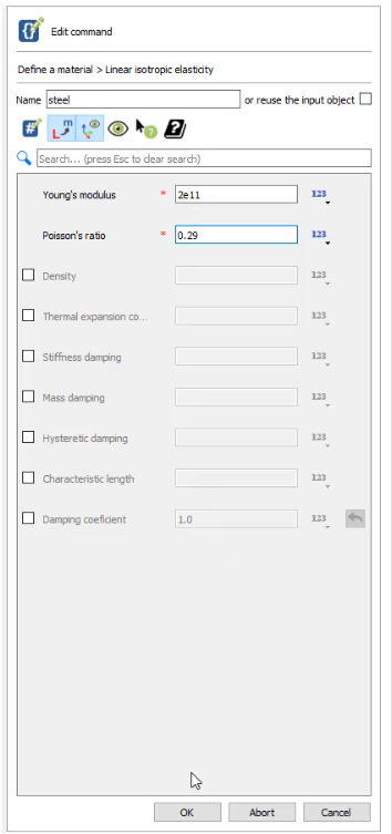
So in this case I used 2e11 Pa as the value for the Young’s Modulus and 0.29 for the Poisson’s ratio. Because I don’t have gravity in this I don’t need to enter the “Density”. Done for my material.

Now let’s start “Assigning material.” So now that I have defined it, I need to assign it to my model.

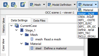
So you have two ways: You can assign to the “Mesh” or assign it to the “Model.” I didn’t create the model yet so I’ll choose to assign the material to the mesh.

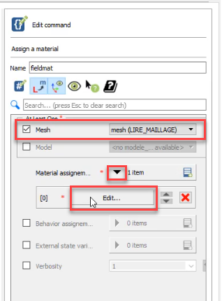
Then click on Edit to choose how to assign the material. Choose “Everywhere: Yes” to assign it to the whole mesh set.

Then choose “Mechanic” as the Phenomenon studied and add a new “3D” Modelisation to the elements of the mesh.

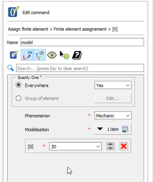
Click on OK and the model definition is done.

Now I have to assign the boundary conditions and the loads. Go in the “BC and Loads” Menu and choose: “Assign mechanical load.”

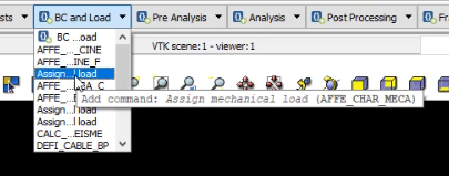
And now let’s assign this to my model. You will see these are many types of loads which are available.

Let’s select “Enforce DOF (degree of freedom)” which will allow me to fix some degrees of freedom in my model.

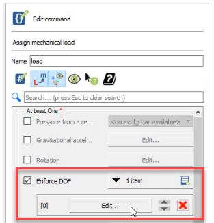
Click on edit and choose a group of elements that you want to fix (That’s where the mesh groups created previously become actually useful).

Select the group “Fixed_face” and click on OK.

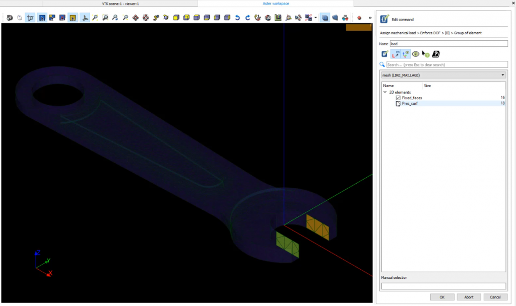
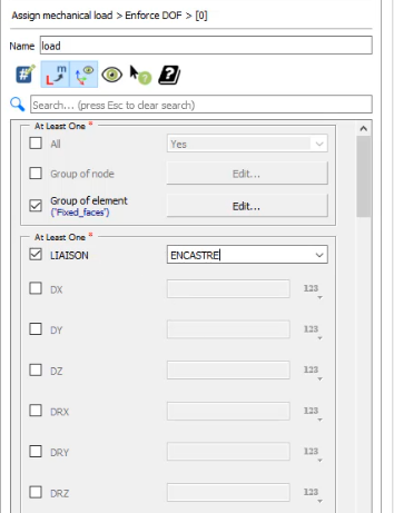
You can choose to fix each of the 6 individual degrees of freedom (DX,DY,DZ,DRX,DRY,DRZ) if you want… but the easiest way to fix all of them at once is just to choose LIASON: ENCASTRE (LINK:FIXED in english).

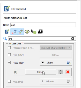
Now that the model is fixed, I want to assign a pressure load. Let’s use the search bar and input “Press”. This will filter out the list of loads and show only the pressure loads available.

Let’s choose PRES_REP as the pressure load (REP is for REPARTITION (French) which means “Distribution”). Check the documentation if you want to understand all the types of loads available.

Then choose the right mesh group “Pres_surf” (or whatever you called it in your model).

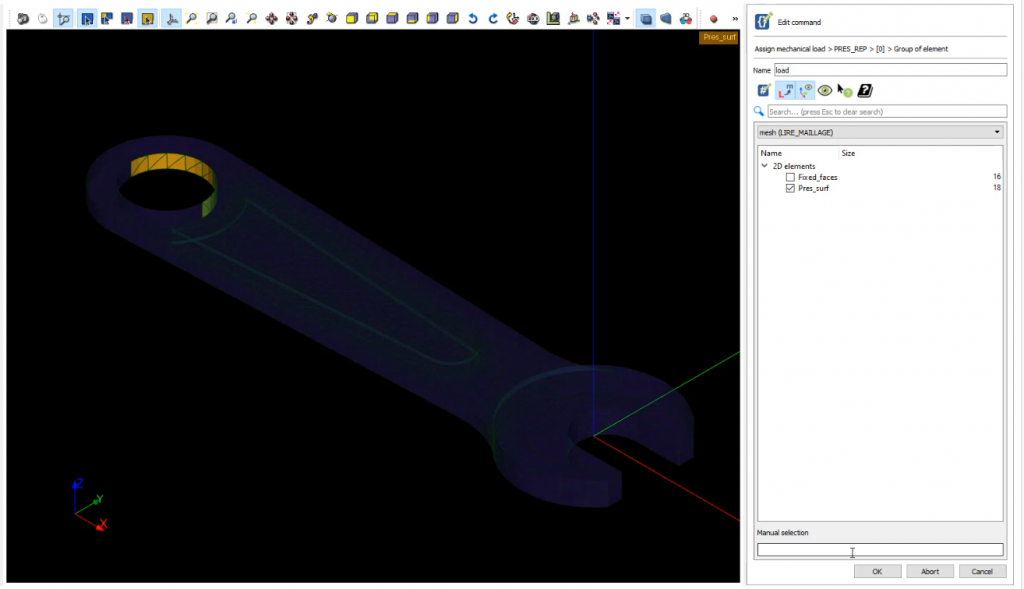
You can then enter the pressure value in Pa unit. So in my case, the value will be 10000000 Pa.

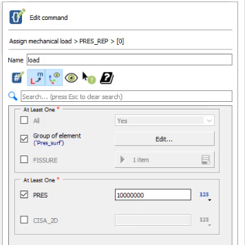
Okay, so the loads are assigned. Now I’m ready to assign my analysis case. So Code_Aster supports several types of studies: Static, Dynamic, Modal, Thermal,…

This analysis will be a linear static analysis, so go in the Analysis Menu and Choose “Static mechanical Analysis (MECA_STATIQUE)“:

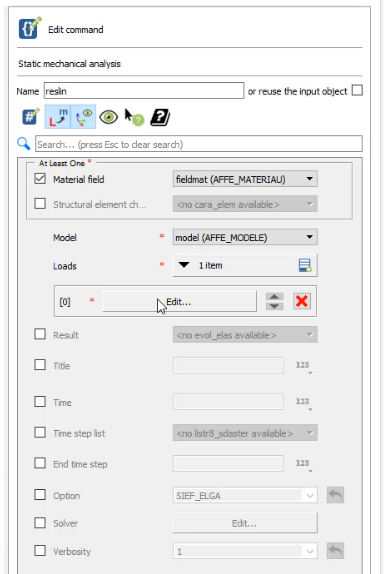
Select the “Material field.”, then select the “Model.” Add a new “Loads.” item and click on “Edit”:

You have some option if you want to multiply the load by some function or this kind of stuff. I don’t need that. Just click on Ok.

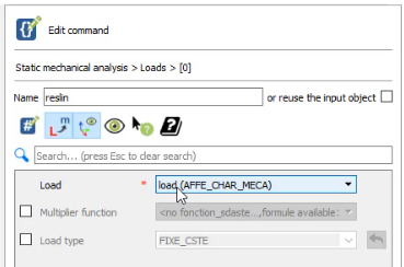
This is all you need to define the analysis case.

By default, the analysis only calculates the displacements at nodes. So if you want to have additional type of results, like stresses, stresses on nodes, Von Mises stresses, you have to add a Post Processing command called CALC_CHAMP, which will, basically, tell the analysis case”Okay. I want more results than just the displacements.”

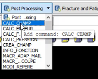
Make sure the name of this command is the same as the analysis case or it won’t work… this is a classic mistake for beginners (So I can either change the name to “reslin” here or check the “reuse the input object” checkbox).

Now I can choose what type of additional results I want. So if I go into CONTRAINTE, which means “stress” in French, I can add some kind of stresses. And, here again, those notations can seem very strange and you have to understand what they mean.

So first of all, you see, you have “EFGE.” You have “SIEF.” You have “SIGM” and you have others. You need to check the documentation to knwo the subtle difference…I just know that this one, “SIEF,” is pretty useful, and what it means is that, I think, SIGM means sigma. it’s the scientific notation of the stress. In French, the stress tensor is generally noted as Sigma. The EF means “efficace” in French (“efficient” in English), so sigma efficient. And you have three types of results every time. You have ELGA, ELNO and NOEUD. So ELGA means that the stress will be given at the the Element Gauss Points.

So in conclusion SIEF_ELGA will give you sigma efficient at the element GAUSS points. SIEF_ELNO will give you sigma efficient on the element surface and SIEF_NOEU will give you sigma efficient at the nodes.

Similarly, SIEQ is the short name for Sigma Equivalent at this will give you all kind of criteria useful to assess the stresses such as Von Mises and Tresca stresses for example.

Check all those results as the image below and click on Ok.

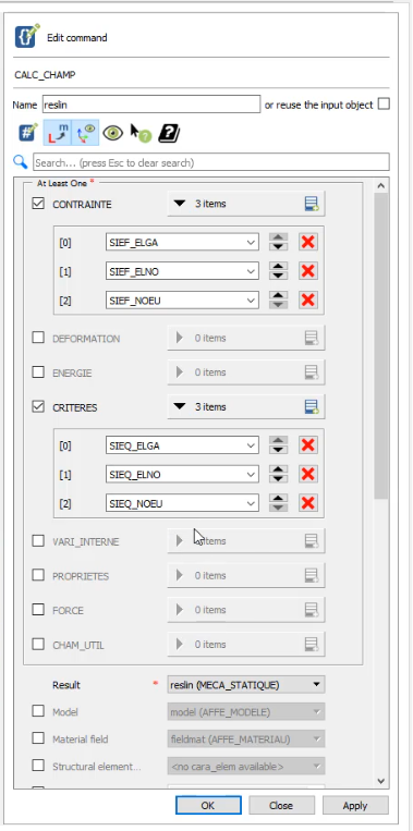
One note is that if you want only the stress nodal results, you can’t just select SIEF_NOEU, you have to select also SIEF ELGA and SIEF_ELNO. This is due to the fact that the field at the node will use the results as gauss points and element nodes to be calculated.

Now I’m almost done. I still have one step, which is to save the results into a file. There is a command for that called IMPR_RESU, which set the output results.

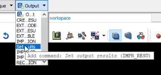
And here I have to choose the format. So I’ll use “Med format,” which is the format of the results that will allow me to read the result within Salome Meca within the Paravis. Then click on the 3 dots and create a new file called “wrench2.rmed” which will contain the results in med format.

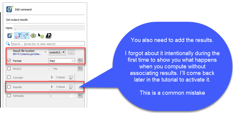
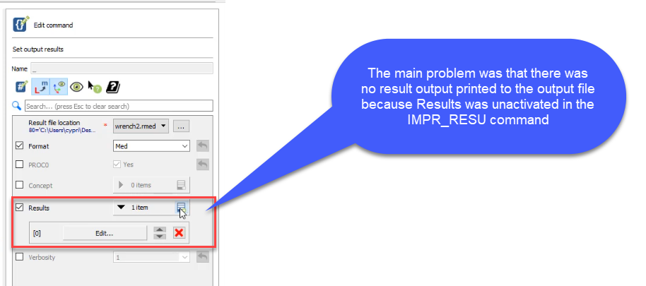
You also need to add results to the file, otherwise the file will be blank. but as this is a common mistake to forget that, I’ll just leave that uncheck for now just to show you what happens.

Step 4 – Computing the results with Code_Aster

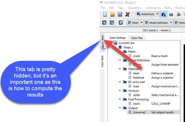
To calculate the results you have to switch and go into the “History view.” So there’s a tab at the top left of the tree which is a bit difficult to see but this is actually important.

There is a “Case view” and there is a “History view.” That’s how we switch to the actual “Solver running interface.”

You have the “Current case,” which represent the current analysis case you have setup. If you already have run some simulation you’ll see some cases which are already below that.

Click on the green cross to add a calculation stage and click on the button called “Run” at the bottom.

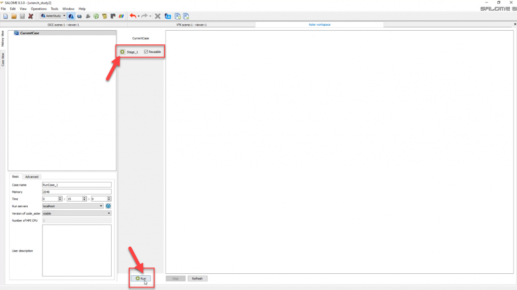
While the solver computes you’ll see in the window at the bottom a “Message file,” which will, basically, indicate to you what is going on.

So the solver will go through all the commands into your command file (what we defined previously) and it will tell you if something went wrong or if it is calculated.

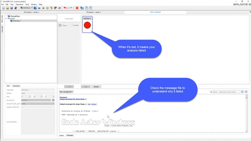
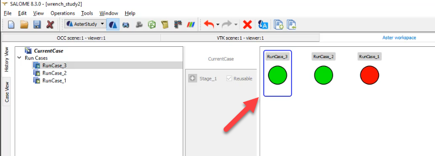
So if you see a red circle like that, it means that you have a problem somewhere in your model and it wasn’t able to calculate.

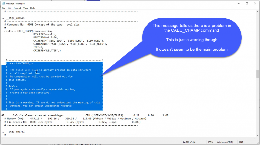
So then you go down until the end and you just look at what is actually the problem here? Okay, so here it tells me that, “The field SIEF ELGA is already present in the data structure at all required times.” So I won’t need this. So I put it two times SIEF_ELGA, SIEF_ELNO, SIEF_NOEU. So it’s … Yeah, maybe I don’t need to put it two times. But that’s just a warning.

In this very cases, it’s difficult to see what really went wrong because it looks like the calculation was finished without any major error, but the circle is still red.

Now… I have already told you that I did an error on purpose. I didn’t assign the RESULTS in the IMPR_RESU command, so the problem here comes from the fact that calculation is finished, but no result is really written.

Let’s go back to the “Case View” and correct that by adding again those results:

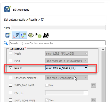
Now, click on OK, go back to the history view and re-compute:

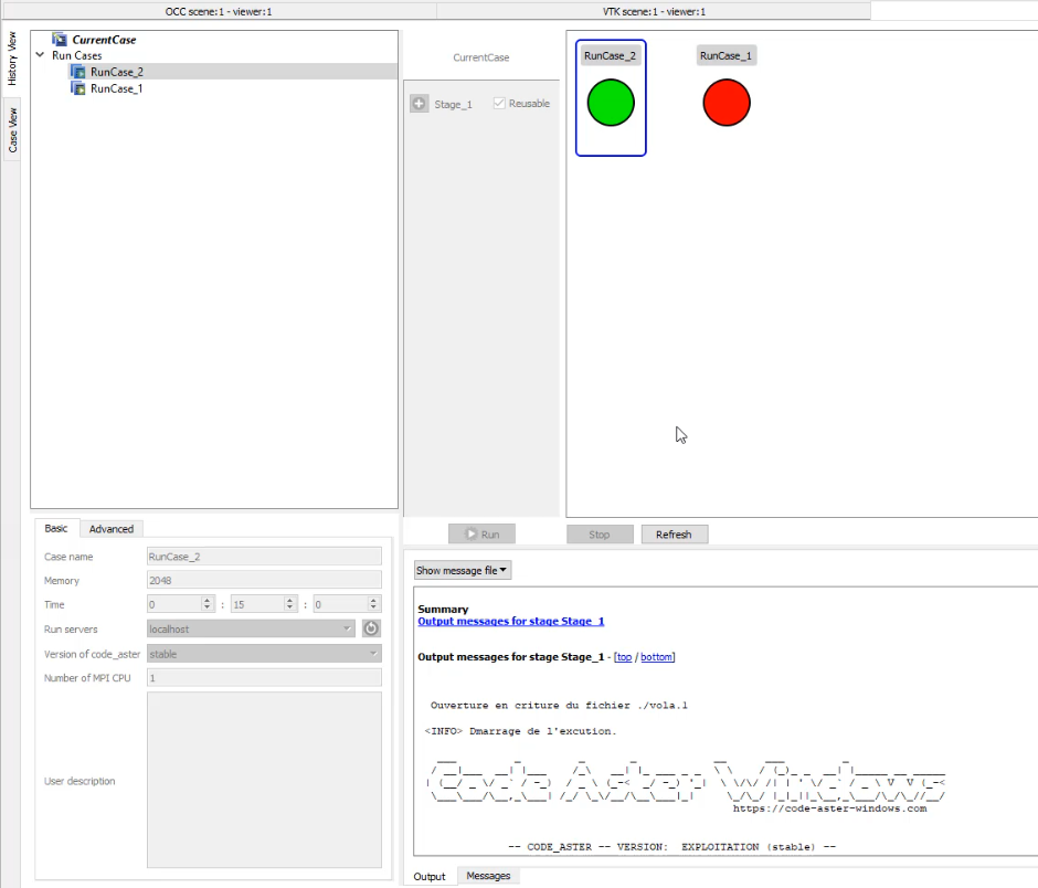
Now, I get a green circle, so this means that everything has been correctly computed.

Now we are ready to look at the results.

Step 5 – Post-processing the results

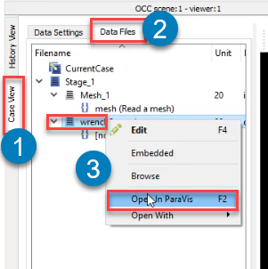
Let’s go back into the “Case view.” And to look at the results I have to open them into Paravis.

Click on the “Data files” Tab. This is where you’ll find the files which are linked to my study.

You should see your result file “wrench2.rmed” listed here. Right click on it and choose “Open in Paravis”.

This will automatically open the Paravis module and load your results:

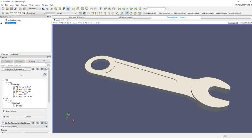
Now I have opened my “Geometry.” Let’s have a look at the properties which are within this file.

You can see all the results which are saved into your file in the properties window. So in case you don’t have anything here and you’re wondering, “Why I don’t have any results?” then you’ll have to look here and see if those results are actually present here. If they are not, that’s probably because you forgot to assign the results in your CALC_CHAMP command.

Another common mistake as I mentioned before is to to leave the default name of the CALC_CHAMP command… remember, CALC_CHAMP needs to be renamed as “reslin” (if your Analysis Case is called reslin).

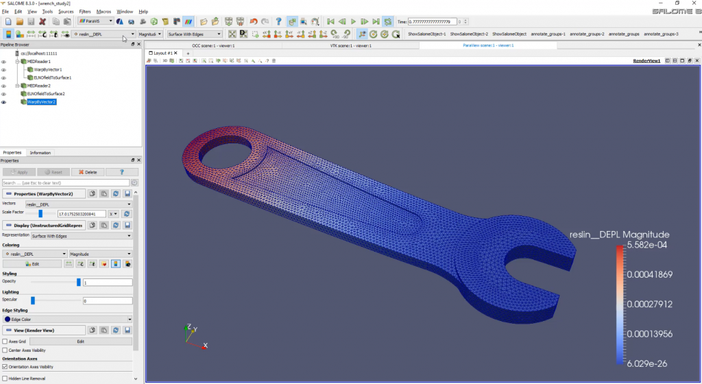
Now let’s have a look at the displacement magnitude reslin_DEPL Magnitude:

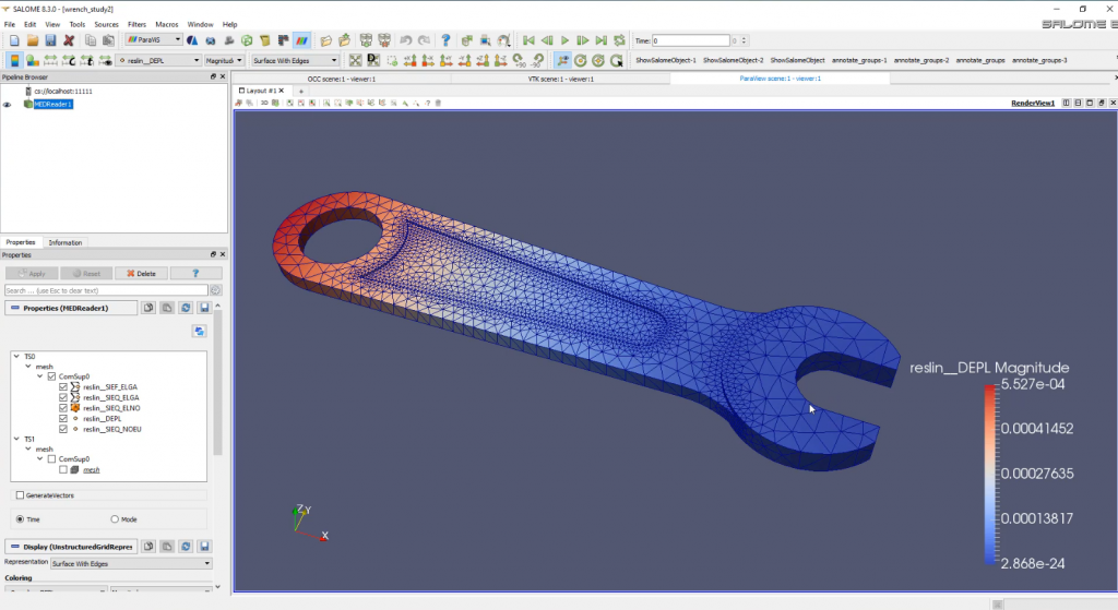
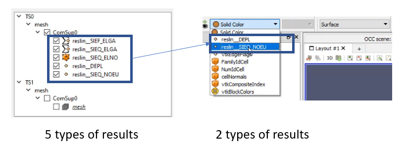
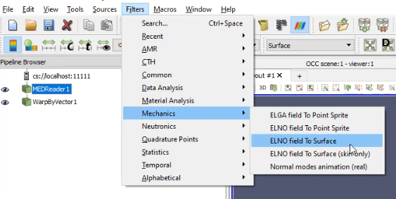
Now, what is strange is that in the properties window, you have five types of results, but in the menu you can only visualize 2 of them. You only see displacement and the stress at nodes because, by default, you only see the “Nodal” type of results. You have to apply a filter to see the other types.

You will find this filter in Mechanics > ELNO field to Surface.

Let’s have a look at the Von Mises Stresses at the nodes:

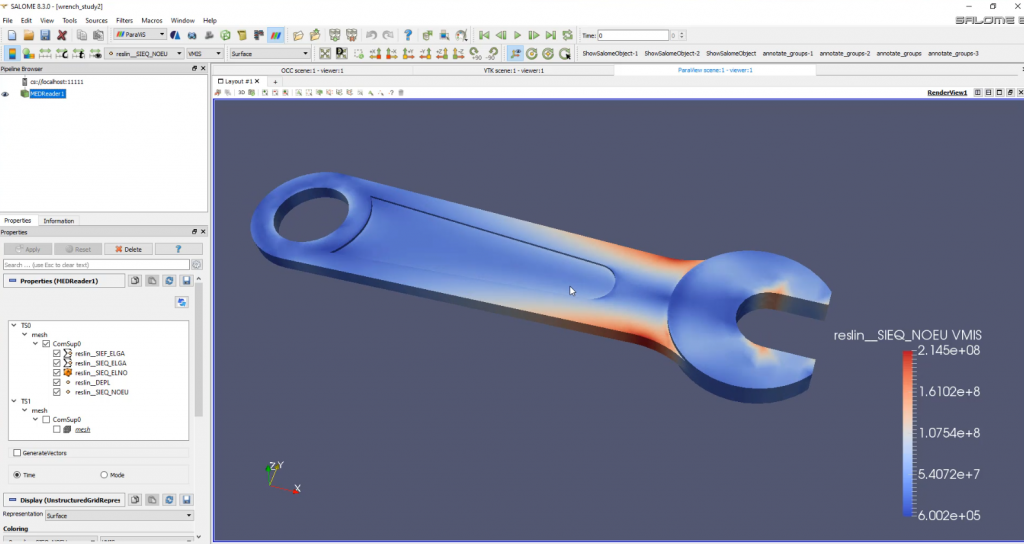
Let’s view the deformed shape. For that there is 2 steps:

• Check the “GenerateVectors” box below the results in the properties window
• Add a Filter > Common > Warp by Vector

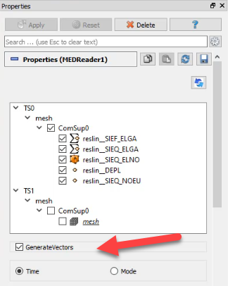
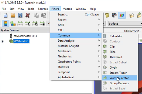
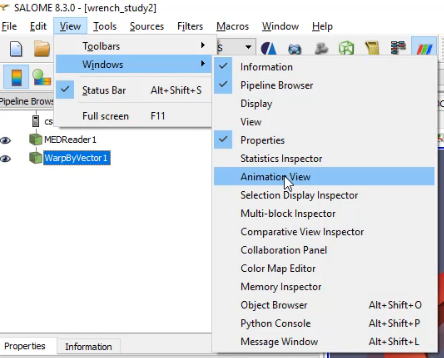
After you did that, you can animate the deformation by doing the following:

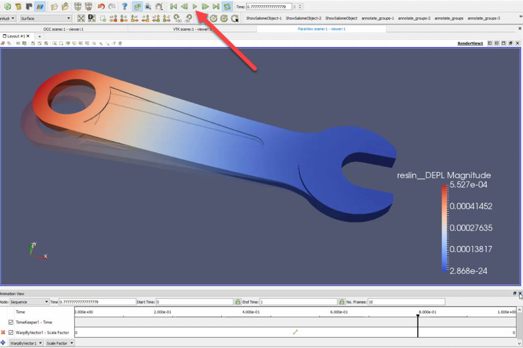
• Activate the animation View (if you don’t see it)
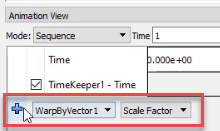
• Choose WarpByVector1 > Scale Factor and click on the “+”
• Click on the play button to see the animation

I have a full video showing how to animate results in my Paraview tutorial series here in case you want to go more in depth.

Step 6 – Discussion about the results

The stress results I was displaying before is averaged at the nodes, so the distribution doesn’t look that great:

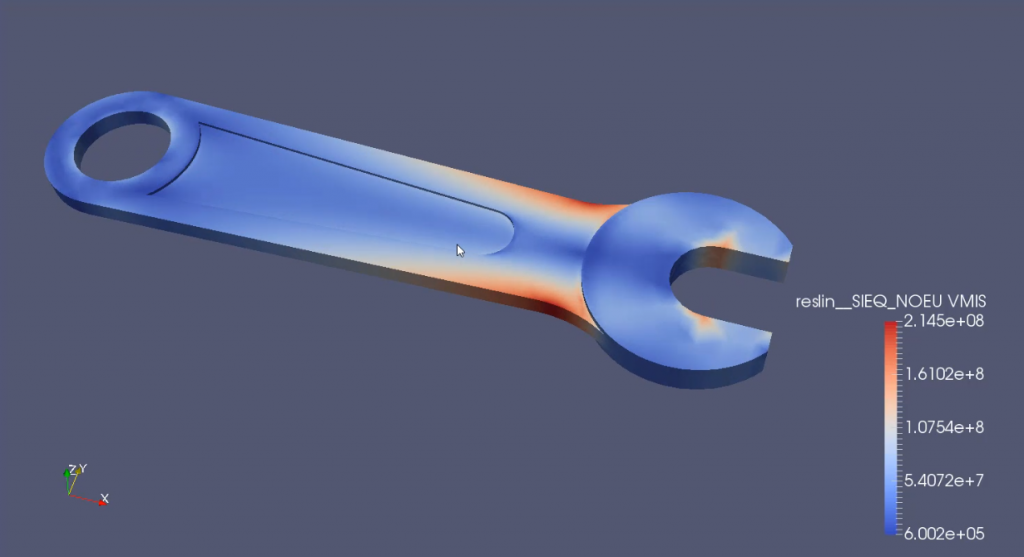
Let’s look at the SIEQ_ELNO (Stresses at element nodes) without averaging to get a better idea of what’s going on here and let’s activate the element boundaries:

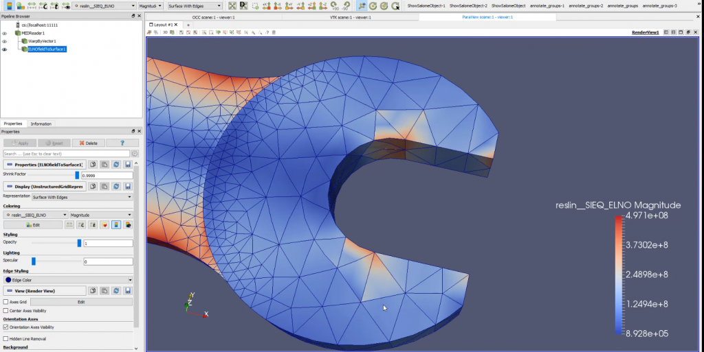
You see very well that this time the distribution of stress is going along the elements and not along the nodes because you have some discontinuity in between the elements.

Stress are always calculated on the elements. It’s an elemental type of result field. It’s not nodal field. So whenever you get a nodal distribution of stresses it’s always an approximation. There is an averaging of stress at the nodes. If something wrong is going on you won’t necessarily see it in the averaged results.

Okay, so now let’s have a quick think about how to refine this mesh because I don’t like it very much. It really doesn’t give me very good results. So let’s go back to my meshing module and let’s have a look at how to re-mesh.

Go back in Smesh, edit the hypothesis of Mesh_1 to setup a Max. Size of 0.002 m and Min Size of 0.0008 m (I tried several times to get a good looking distribution not too fine and not too coarse)

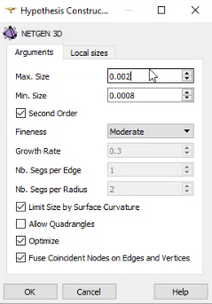
That’s what you’ll get:

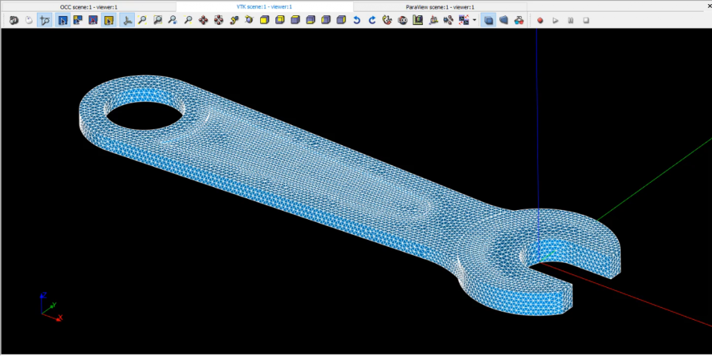
Don’t forget to recreate the mesh groups using “Create Groups from Geometry”.

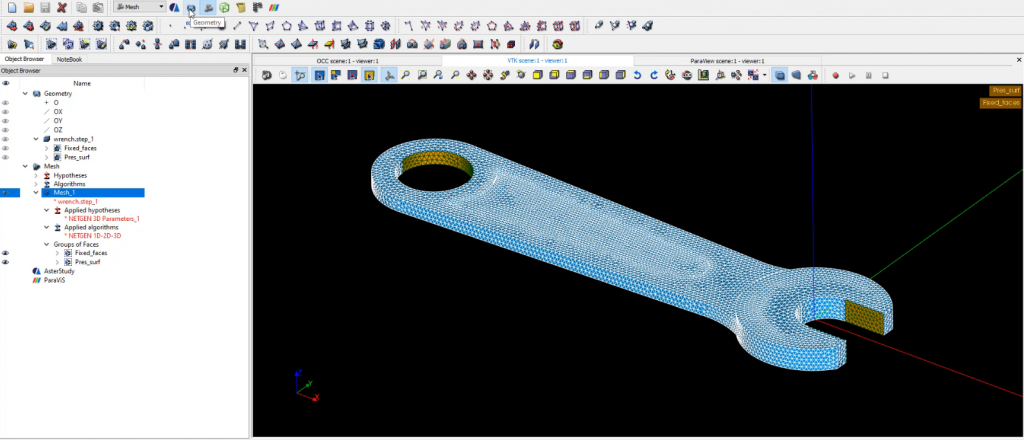
And now, I would say, I don’t have much more to do. I just need to go back to the Aster_Study module. Make sure your model is loaded again. So I don’t see it anymore here. It has disappeared, and that’s because I changed the mesh set.

So what I have to do is just double click on the “Read a mesh,” to re-read the mesh, and you see the name hasn’t changed, it’s still the same, so your model will automatically be loaded again, and it should be fine.

Then Re-compute the results and get green again (hopefully)

The results are now looking much better as the mesh has been refined:

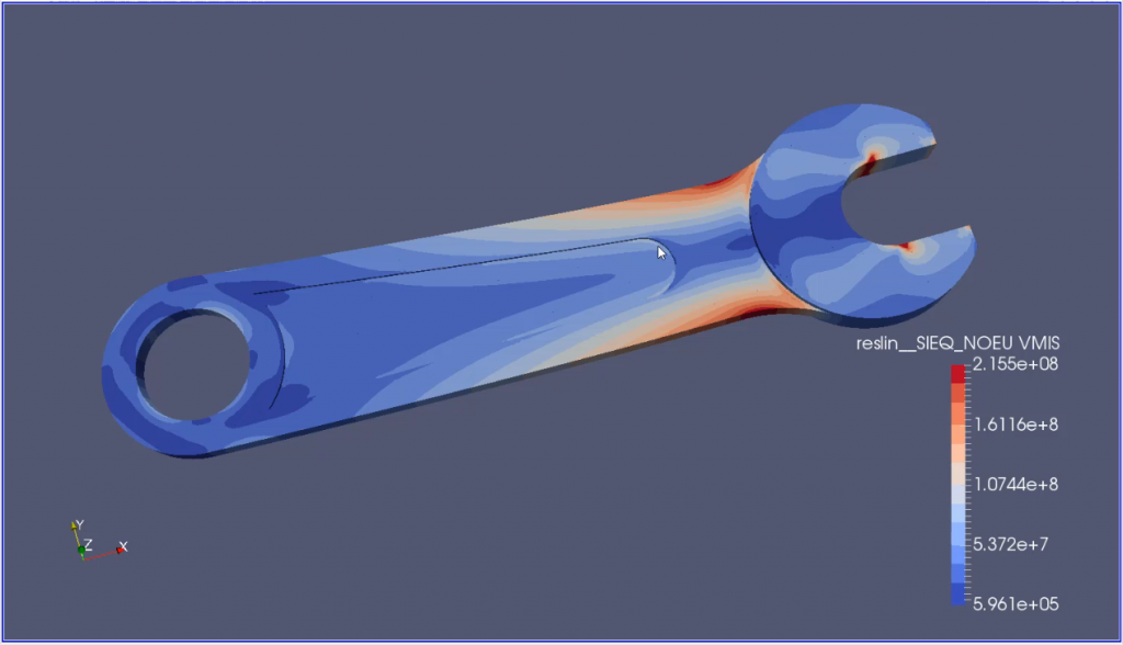
Let’s have a look at my Von Mises stresses. And this time the mesh distribution looks better. Let’s change slightly the colors, and for that let’s activate the Color Map View. Let’s decrease the number of color to 12.

If you look at the colors like that, especially if you have few colors you’re better able to see where higher stresses are concentrated.

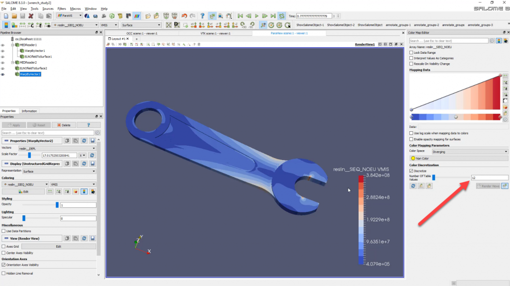
And you can see here that, in this case, I have this small region here where there seem to be an accumulation of stress.

This is called a stress singularity and this is probably just due to the fact that I fixed those surface and there is just a discontinuity of the degrees of freedom in between, which generate this kind of singularity.

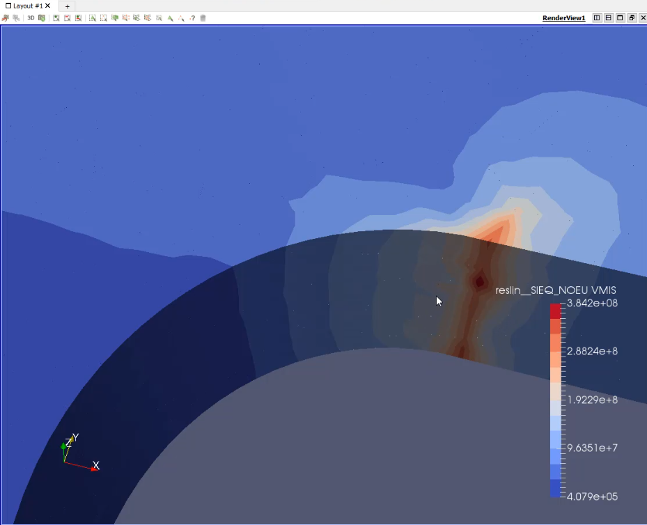
This stress singularity means that I cannot really trust all the results near the singularity as being the real maximum Von Mises of stress in this model. This is probably just some kind of artifact and we can ignore the stresses in this region.

But how do you know which are real stresses from which are not?

Let me show you a quick method I found out:

• Select the whole model elements
• Unselect the region of high stresses near the singularity
• Extract those elements in a new set with the Extract Selection Filter
• Rescale the legend

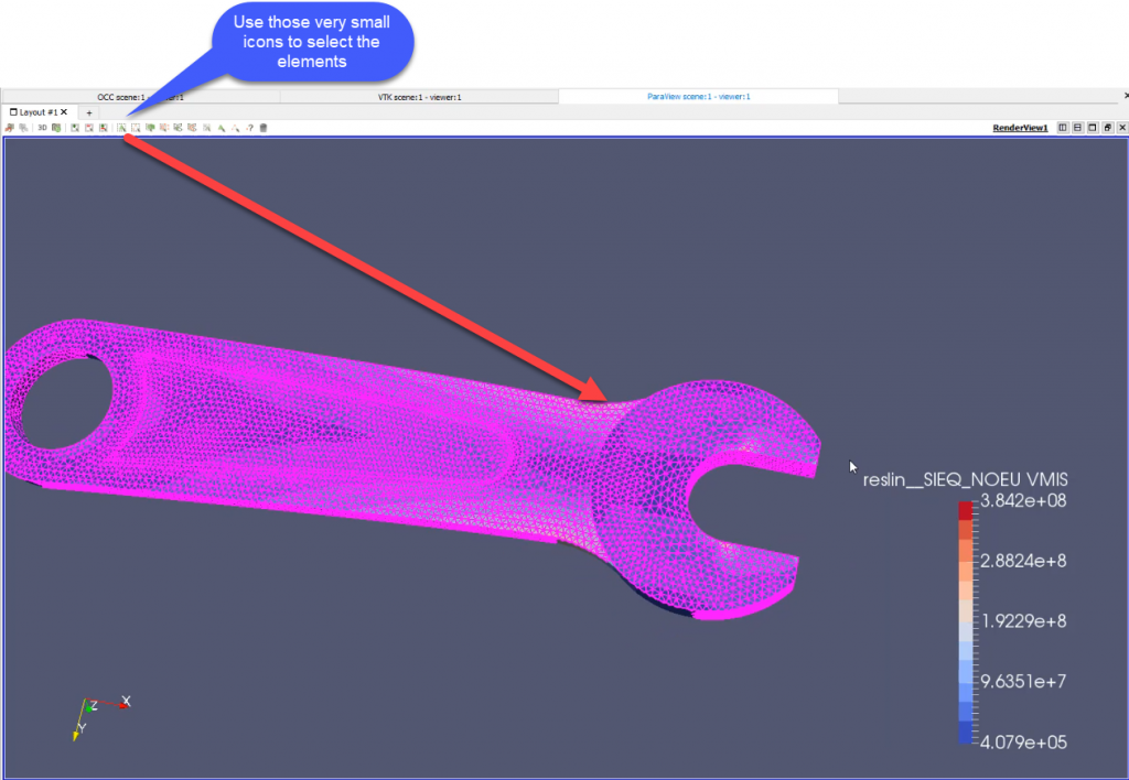
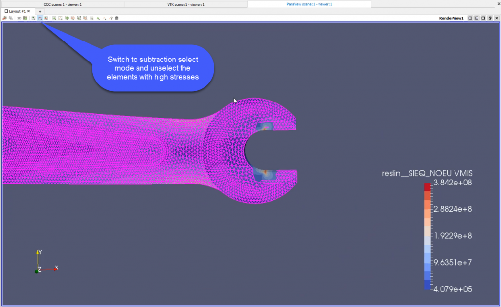
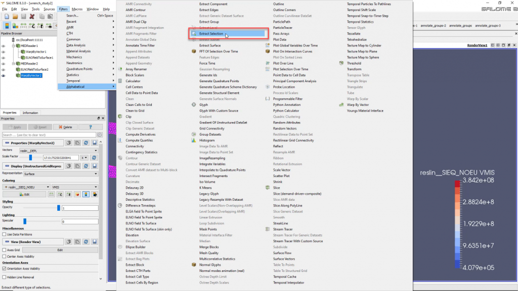
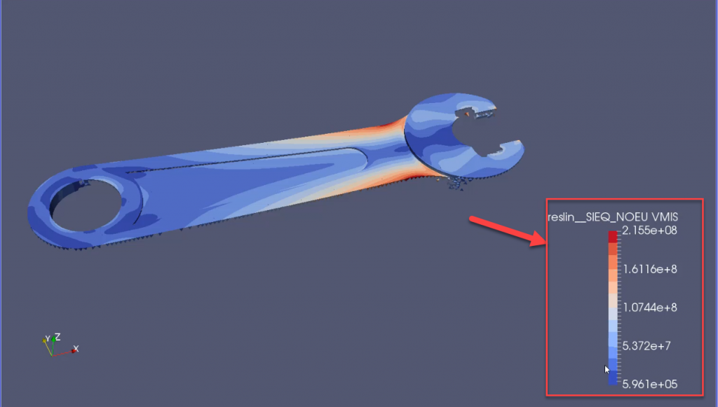
You can now use this rescaled legend to display your previous results in a much more realistic manner:

---

Ok, Guys, that’s all for today… I realize that’s a lot to digest, I hope it was useful.

If it was, please share it with your friends and colleagues and give a like to the video!

Let me know in the comments what you think and what you want to see next!

Cyprien “Wrenching your way into Open-Source FEA” Rusu