Today, Let’s talk about uncertainty quantification and sensibility analysis!
There is an open-source tool for that called OpenTurns which is integrated in Salome_Meca 2019 (Linux version).

There are few tutorials available yet showing the full simulation with Code_aster and the usage of this simulation data to build an openturns case!
That’s why one of my readers, Fernando Oleo Blanco (Irvise) sent me a great video showing exactly step by step how to:
- Build a simple Code_Aster study of a loaded 3D beam
- How to export that study into an Openturns study
- How to analyze the results
Very eye opening and and extremely useful tutorial for the Code_Aster/Open Source FEA community.
Tutorial in Video
A big thank you to Fernando Oleo Blanco (Irvise) for creating this tutorial video!
You can contact him at his email irvise (a_t) protonmail (d_o_t) com if you want more details about his Openturns tutorial.
Step by Step Tutorial
In this tutorial, we are going to be focusing on how to interface Code Aster and OpenTURNS to do uncertainty quantification or sensibility analysis.
For this purpose, I will be using Salome Meca version 2019 However, the 2018 version also allows and has an automatic support of a Code Aster case into OpenTURNS. It is important that you notice that the OpenTURNS module is not available for the Windows version, so you won’t be able to follow this if you’re using the Windows installation of Salome Meca.
Another point that’s important for you to know, I won’t be focusing too much in the geometry meshing and basic case setting in Code Aster, mainly because that’s not the goal of the tutorial, which is to focus on the specifics of Code Aster that need to be done in order to export it to OpenTURNS and then do a simple and quick demonstration in OpenTURNS.
Therefore, I will be going quite fast during the geometry meshing and basic case preparation. So if you feel overwhelmed or where you think I’m going too fast, please feel free to check those basic Code Aster tutorials first.
1- Setting up the Geometry in Geom
we need to set the geometry first in the Geom module in order to generate our case.
It’s going to be very simple. The goal of this video is not to focus on a complex simulation. Therefore, we are just going to create a simple beam. Let’s do that.
Open the Geom Module first:

Let’s create a box.
I’m going to be using the international metric system, called also SI units, and therefore everything will be in meters, pascal, and newton.
So let’s give this some realistic measurements:
- DX is going to be 0.3 m
- DY is going to be 12 m
- and DZ is going to be 0.5 m
Apply and close.

With “Box_1” selected, make sure that you click on the fit selection button, which is this lens and a cube under it so that it zooms automatically into our object.

Then let’s create some geometry groups.
Right-click on “Box_1” , then choose “Create Group”.

Let’s create the load face.
Well, first let’s create the fixed face. Select the face that’s at the origin, add it, and create the fixed face.

Let’s create now the loading face. Select the opposite face of the beam, add it.

Then we are going to create two edge groups mainly to help us with the meshing.
We are going to create the DX group. You can choose whichever edge is in the DX direction, add it.

Repeat for DZ direction, choose whichever edge you want in Z direction, apply and close.
Before we continue, don’t forget to save the case (Because you never know…)

2- Setting up the mesh in Smesh
Let’s get into the meshing section of the tutorial.
Open the Smesh Module:

Select the box, and click on Fit to selection to have it in full screen.


If everything went well in the previous geometry creation step, you should be able to see the 4 geometry groups: Fixed, Load, DX, DZ just below the Box_1 Item in the Object Browser (Or whatever name you chose to name them).
Now with box selected, let’s create a mesh.
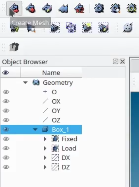
Choose “Hexahedral” as the mesh type.
Then assign the set of Hypothesis “3D: Automatic Hexahedralization”

Then Choose 100 segments in the “Hypothesis Construction” window that pops up:

Apply and close.
With “Mesh_1” selected, let’s create some submesh.
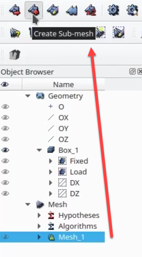

- From the geometry, we are going to select DX.
- It automatically sees that we are selecting an edge, and gives us the 1D option.
- In algorithm, we are going to give it a wire discretization.
- In hypothesis, we’re going to add the number of segments, which is going to be 10.
- Okay. Finally, in additional hypothesis, let’s say we want that same hypothesis propagated to all the opposite edges
- Apply
Let’s do the exact same thing with the DZ edge group.

Salome automatically fills the same hypothesis that we have just created, so we just hit apply and close.
Let’s generate the mesh now.
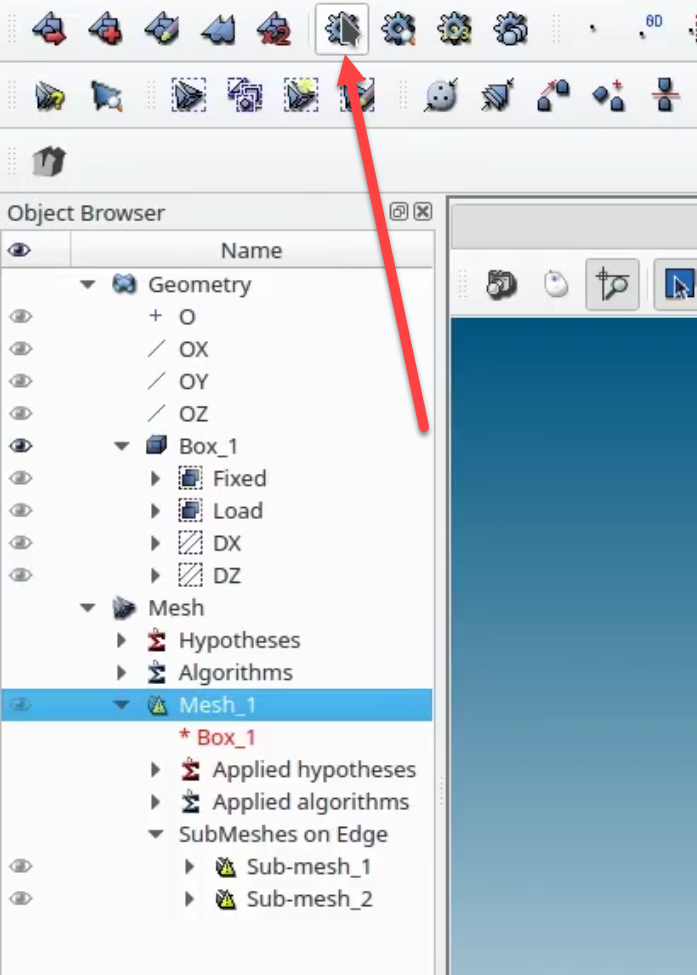
Select mesh 1 and compute the mesh.
We can see the mesh that it has created:

Now with mesh 1 selected, let’s create two geometry groups. Those will be our fixed face and the loading face.
Create group. We’re going to create group of faces, group from geometry, direct geometry selection. Let’s select our fixed group and let’s name this group fixed, apply.

Let’s call this next group load, and let’s select the load face.

Apply and close.
If you would like to see those two, just click on the icons and you will see them.

We will come back later to do another group, but for the time being, let’s just make sure that we are running a successfully running case.
We will add a final group that we will be using to do the uncertainty quantification. Let’s save the case.
3- Creating the Code Aster Simulation Case
Let’s go into the Aster Study module and let’s set a very basic simulation case.

Once again, I won’t be explaining everything with great detail since this is not the goal of the video. Add a stage.

With our stage 1, let’s just start creating a very basic simulation.
Mesh>Read a mesh:

Make sure there is a mesh item selected in the Mesh and then let’s add a Finite Element Model.
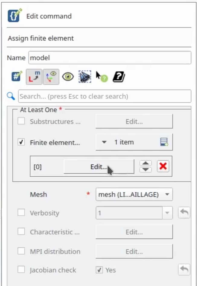
Open Finite element, Click on Edit.
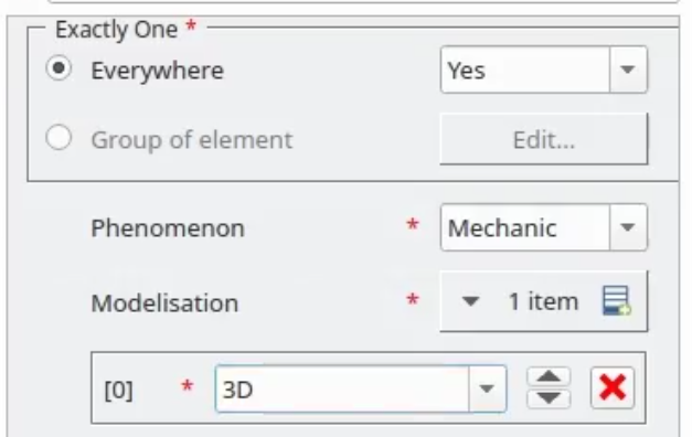
Phenomenon: Mechanic. Although you can just pick whichever one you want for your case, in this example we will be doing a mechanical simulation and we will use a simple 3D Element Modelisation.
In materials, let’s define a material:
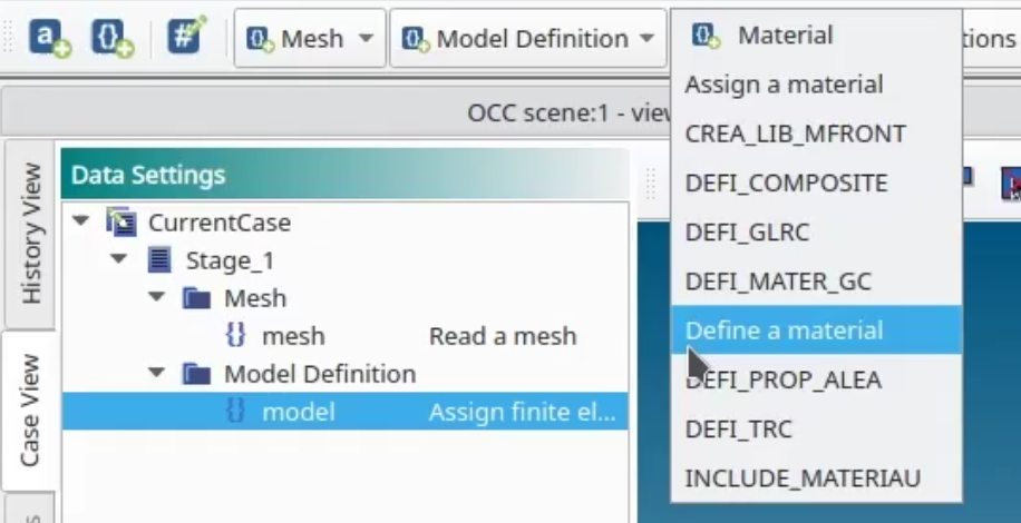
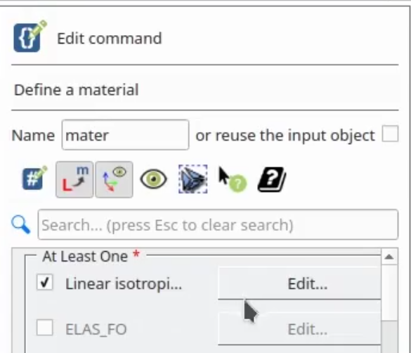
Choose the Linear isotropic material model and click on Edit:
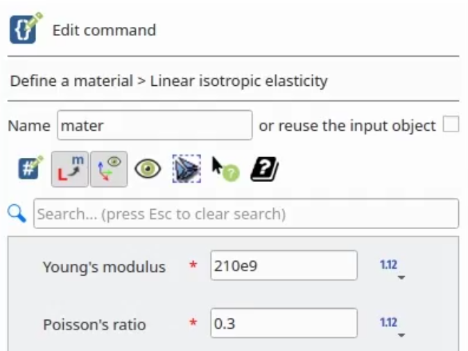
Set the Young modulus to 210e9 and the Poisson ratio to 0.3. Call this material “steel” and click on Okay.
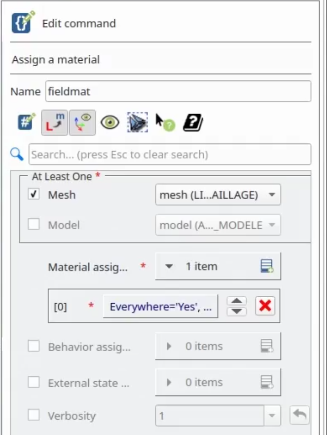
Let’s assign the material to our beam or mesh.
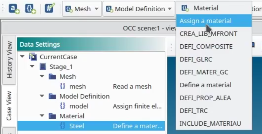
Now let’s create two boundary conditions which are going to be our fixed face and our load face.
Let’s now assign the mechanical loads:

Name is “Fixed”, then check the “Enforce DOF” Item and click on Edit:
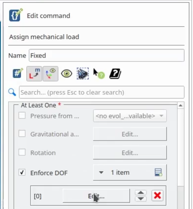
We now need to choose the Groups of Elements whose degrees of Freedom will be constrained. Choose “Group of Element” and Edit:

Activate the LIAISON (French work for Link) and Select “ENCASTRE” (This means that all DOFs will be constrained).

Click on Okay.
Now let’s create the load. Assign mechanical load, and we are going to scroll down till we get to force face.

Select the Group of elements as load. Let’s give it a value of -37 kN down in FZ direction.

Now in analysis, we want to do a static mechanical analysis:

In the material field choose the fieldmat object we created before, which contains our assigned material. The model should be automatically set as the model we created before too. Click on the icon at the right of the Loads to add our loads:

On loads, we want to add both loads: the fixed load and the load0 load. Click on Ok.
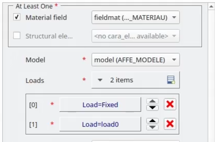
Now that we have created our simulation case, let’s see if it works correctly. In order to do that, let’s click in history view:

at our stage, and click run.

The case runs to completion, which means it is set up correctly:

Now we can focus on the specifics on how to get it to work with OpenTURNS!
4- Setting the model for Openturns
The case that we are going to see in this tutorial, it’s a very simple case and we are going to do a very, very basic uncertainty quantification analysis of how much deflection the beam suffers depending on the load and depending on its Young modulus.
In order to do that, we are going to add a node group.
Go back to the smesh module:

let’s open the mesh, mesh 1, and select it.
With the mesh 1 selected, let’s create a group:

It’s going to be a node group and we are going to call it Node1.
Select enable manual selection and select whichever node you want from the lower section of the beam, Add it. Apply and close.

Let’s go back to Aster Study, case view, and let’s save the case.

Now, in order to generate a Code Aster case which can be used in OpenTURNS, we need to export that data, the result data of our simulation, in a format that OpenTURNS will be able to interpret.
To do that, we are going to create a table. In order to create a table, we need two different functions. The first one is in post processing and it’s called POST_RELEVE_T. This function will allow us to extract data from our simulation. In action, let’s add one.

We are going to stack a result from the reslin simulation case created previously. Let’s create a new Action:
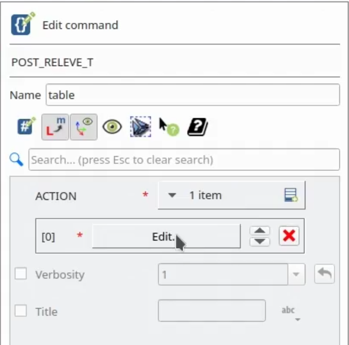
In operation, we’re going to do a simple extraction.

That extraction is going to happen from a group of nodes. That is why we created our node group, which is just going to be this simple dot over here.

We need to select what do we want to extract from that node. I’m going to extract one of its results, and it’s going to be the DZ displacement.

We are going to see how much it will drop after a load and the Young Modulus is applied. We can give it any name: Let’s call it displacement. The name of the field, it’s going to be a displacement field, so DEPL, then click okay.

Now we have created our table. In order to output this table, we need to create an output table. That is done in the section output, IMPR Table, which I suppose means imprint table. Click on it.

In the table field, we want our table selected. Since we only have one, it has already been selected automatically for us. We need to create a file name. So click on those three dots and let’s add a file and name it in like you want.

But you have to add the npy, extension to the file. So I’m going to call it dz_table.npy. Let’s save it.
In order to see what is being output, click on the format and leave it at tableau.
This is not correct and this won’t work with OpenTURNS. However, we are first going to run a simple simulation to see the information that’s been output into that table.
It is also very important that you name your parameter. It’s not required when we are running the tableau option, but it will be very important if we are running in an OpenTURNS simulation. We are going to call our parameter DZ.

Let’s click okay, and now save the file.
Now let’s see what out IMPR_TABL command will generate into this new file we just created!
Let’s get into history view, select our current case, add it, and run it again.

It has run to completion!
Now, let’s go into our save folder where we saved our case. You should see a file named in whichever way you named your output table. Let’s open it.

Select whichever text editor you may want and look into it. As you can see, we can see the name of the parameter that we have given it and the actual displacement, well, the actual parameter that we wanted to output. In this case, it’s the DZ displacement equal to -4.75E-3 mm

Okay. Great. Now we see that everything is working. Let’s go back into our case view, select our output table command, and change the form from tableau to numpy.

This is the only format that works with OpenTURNS, so it’s very important that you select this one.
I want to repeat myself: it is also very important that you name your parameter. Otherwise, the export function will tell you that you need to give it a name.
Click okay and save it.
5- Exporting the Code_Aster Case to Openturns
In order to export a Code Aster case into OpenTURNS, we just have to go up into our current case, select it and click on it. Here, you can see our export to OpenTURNS.

Let’s click on it. The export dialogue will tell us that we are still missing one thing. Here, you can see it’s giving us a warning, “No Python variable found. You must add one or more Python variables in a graphical stage of your study.”
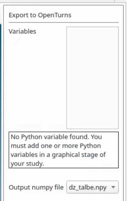
This means that if you have a pre-made case, for example, one that you created a long time ago, the parameters that you’re using within your case need to be turned into variables. These variables are going to be the case input variables in OpenTURNS.
In our case, we are going to change two parameters, the Young modulus and the force that’s going to be applied.
If we select, in our case study, the steel material, double click on it, go into the linear isotropic section that we created earlier and let’s change this number, which is just a simple number.

Let’s change it into a variable. Add a variable.
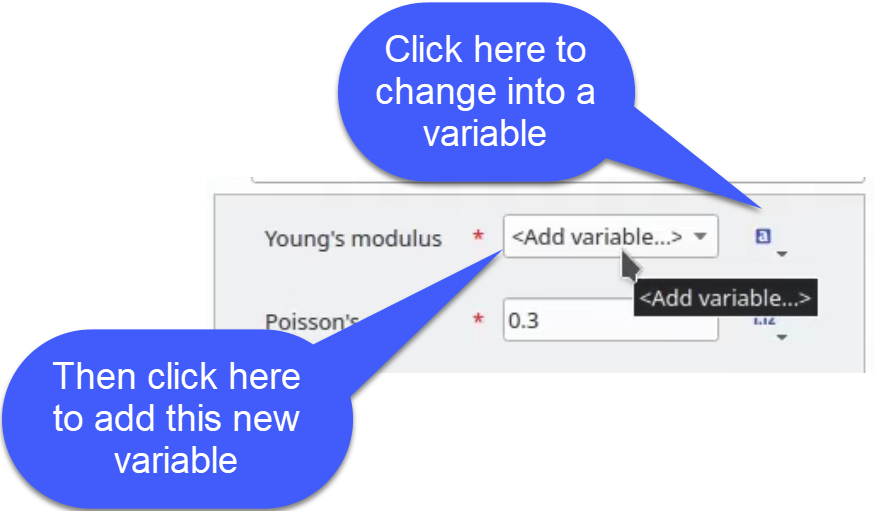
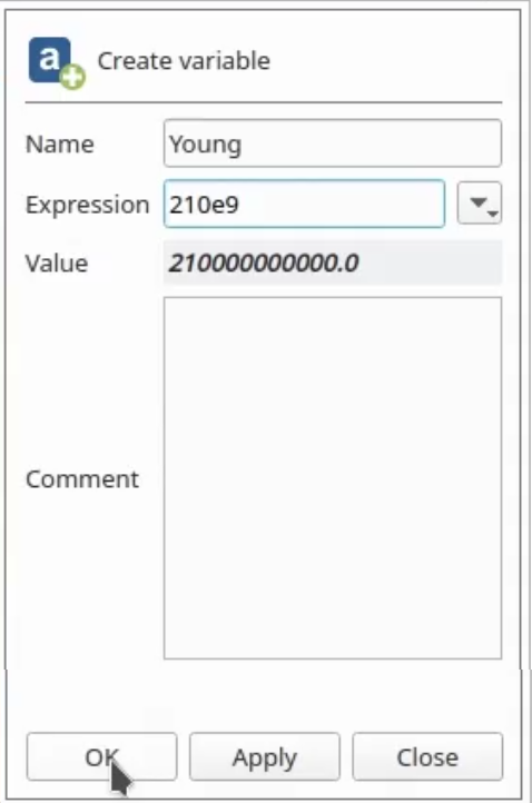
Let’s name this Young. We need to give it an expression. This expression doesn’t need to be a mathematical formula, a simple number will do. We’ll just give it what we had earlier. Okay.
We’re going to do the exact same process with the force. So under boundary conditions and load, let’s select our load, scroll down to where we select it earlier: FORCE FACE, and edit this force.

In the FZ component of the force, let’s change the number into our variable.
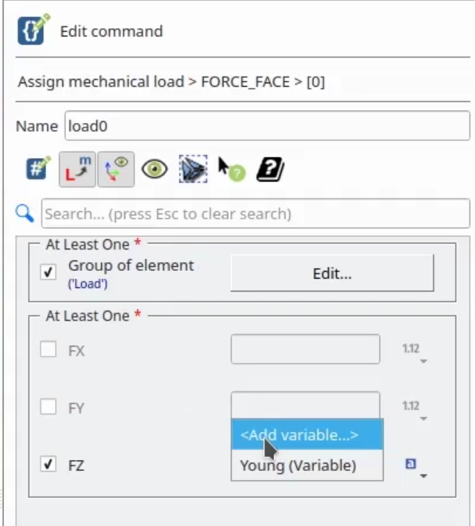
We click on the drop down menu and click on add a variable. Name it force. Under expression, whichever number you may prefer. Let’s say 37 kN.
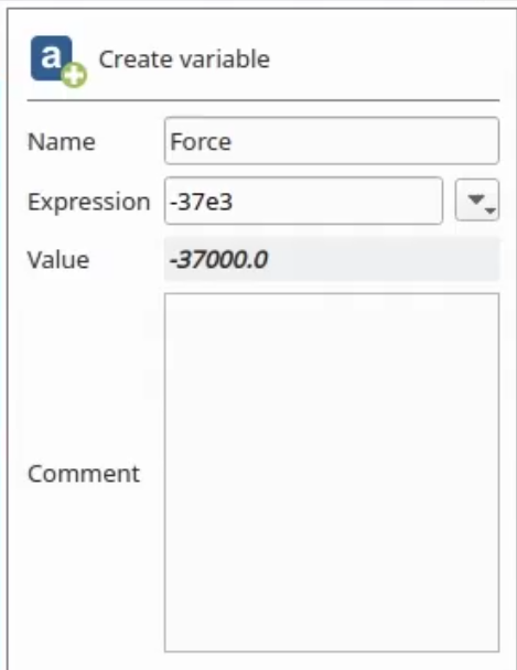
Then click “Okay”.
Let’s save the case one final time. Let’s scroll up into our current case, right-click, and export to OpenTURNS.

This is what you should be able to see now:
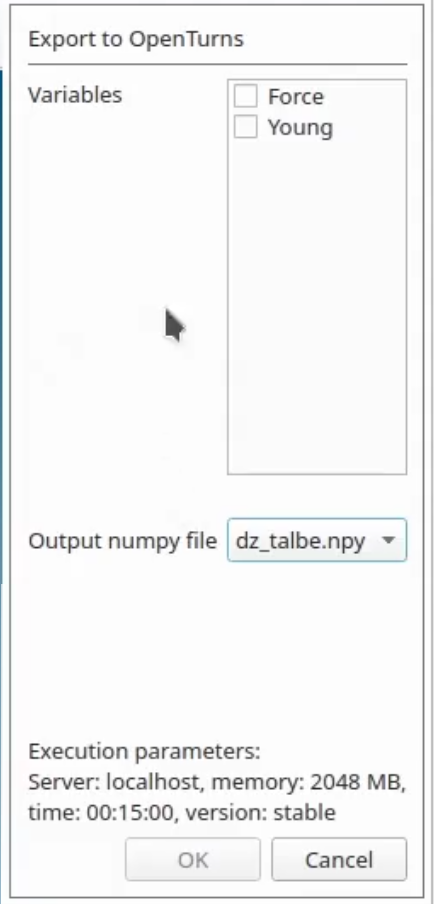
Here in the output numpy file, it has automatically detected that we are creating a table output in the format of numpy. If you did not create a output as a numpy table, it will warn you that you need to create one. In the variable section, we can see the two variables that we have created. These are going to be the input variables that our OpenTURNS case is going to work with.
Select whichever ones that you will want to export as an OpenTURNS input variable. In our case, we are going to select both force and Young, and we can finally click okay.
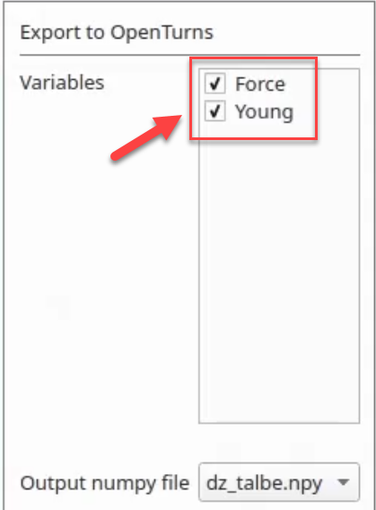
Now, we are automatically launched into OpenTURNS where our case has been automatically exported. Let’s save the case

The screen that you’re seeing right now is the definition screen. This is where our case is being defined. The most important bit in this screen is this YACS model data file. If we click on edit, it will open the Python script that OpenTURNS is receiving from our Code Aster simulation.
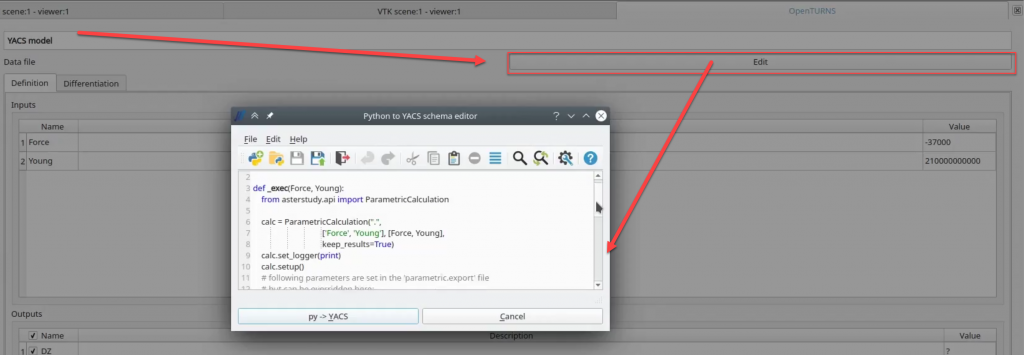
YACS is another interesting module of Salome that can create nice python automation workflows… this is a huge topic in itself, so it will be for another tutorial.
Here in the definition tab, in inputs, we can see our two variables, force and Young, with their preset values that we had added. In the outputs, we can see the DZ output variable and the value right now is unknown since it doesn’t know which is the correct result, since we have yet not run an OpenTURNS simulation for these inputs.

Let’s evaluate it. What we’ll do is start… OpenTURNS will start now its own engine and will run the simulation that we have created in Code Aster. It is going to use a force value of 37 kNand 210 GPa for the Young modulus. With those two values, it’s going to give us the output value.

As we can see, it’s the exact same one we had earlier: -4.75E-3 mm
In order to do a simple OpenTURNS simulation like the sensibility or uncertainty quantification, let’s go into our current case in the left panel. Here, you can see the OpenTURNS graphical user interface.

If you click in model definition, you will be brought back to where we were.
If you click on model evaluation, it will open the model evaluation configuration panel.

Here, you can see it’s exactly the same as we had earlier. However, if you have several outputs, you may turn them on or off or change the input values.

Let’s click on finish. I want to show you a very typical error that OpenTURNS may give you.

Here, you can see the inputs, the force and the Young values. Here, you can see the name of our current evaluation point that we are going to run, and here you can change the number of parallel evaluations that you may want to do at any given time. These are parallel evaluations within OpenTURNS, not the number of the different course that may be used by Code Aster.
If you go into the advanced parameters tab, here you can see some extra information.

This information was automatically extracted from our Code Aster configuration case.
So for example, we had a maximum duration limit of 15 minutes within Code Aster. This time refers not to the maximum time that OpenTURNS may run the simulation, but the maximum time that each simulation, each Code Aster simulation, is allowed to run for.
Then files and directories, we may get…

I will explain them in a bit more detail in another tutorial. These are generated for you automatically when you export the case.
Let’s go back into quick configuration and let’s hit run.

This run will end up with an error like the following:

Error: No results are available. An error occurred during the execution of the analysis.
This error appears because a previous result already exists, since we had already evaluated this point 37 kN and Young modulus of 210 GPa.
That earlier simulation has already created an output directory for those two exact points. This simulation tried to create those exact two points, but it is detecting that they already exist and it’s giving us an error.
If you would like to rerun a previously done point, you have to go to the working directory that OpenTURNS generated.
In my case, is salome workdir Fernando Fernando, etc…. This is the important bit: .run_param_-37000.0_210000000000

This is the directory that we need to delete if you want to repeat a simulation.
So if we go to this directory, salome workdir, you should see this .run_param_-37000.0_210000000000 directory.
If you cannot see this .run param directory, you need to enable hidden directories.
Let’s have a look at what’s in this directory before deleting it:

Let’s open it:

In this directory, you will find the output files that Code Aster generates.
For example, here’s the output simulation file:

You may take a look at it if you would want to understand how it is working. Especially if a simulation within OpenTurns fails, it is quite useful to take a look into what Code Aster is generating.
For now, I’m just going to delete this directory. Let’s go back into our current case:

Here, we can do some screening, optimization, design of experiments, and the final bit we are going to do in this video is a probabilistic model definition.
Click on the probabilistic model definition. Here, we need to define the statistical definition of our input variables. Let’s select both Force and Young.

You can now select the probabilistic distribution you want:
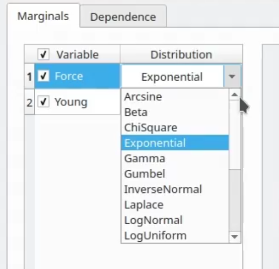
For both, I’m going to select a normal distribution. The proper selection of the probabilistic distribution model is the job of the statisticians… it is pretty complex if you want to choose the right model (Normal distribution is NOT always correct)
Here, in the configuration panel for that very distribution, you can select which parameters are going to be used. Some of them have several types of definitions. Let’s leave them as they are.

It’s not very realistic, but it will show what we want to do.
If you want some more advanced features or a bit of a refinement, you may also add some dependence between those input variables.

We are not going to do that here.
Once the probabilistic model definition has been set up, let’s go back into our current case. We can see that the sensitivity analysis, central tendency, and limited state definition have been highlighted.

That means we can now run them if we want. For this demonstration, we are going to do a central tendency simulation. Click on it, leave the method as Monte Carlo and make sure that our output is select.

Click on Continue.
Now, we need to select some parameters to refine the accuracy of our simulation, the maximum time we are going to let our simulation run for, and this refers to the OpenTURNS simulation not the Code Aster one, or a maximum number of calls, a maximum number of points that we want generate.

I’m going to select a maximum time and I’m going to leave it for 30 minutes. Now, you may want to leave it for less, or you may want to live it for more. The more time you let this run, the more points will be generated, keep that in mind. Now, let’s click on Finish.
Here, once again, we have the configuration panel for our central tendency problem.

I’m not going to change anything. I’m just going to launch the simulation as is right now, and I will let it run till completion.
That means 30 minutes. After 30 minutes of simulation in my case, you will be automatically presented with this new screen:

In this new screen, you will find the results that were generated during all those simulations and a final analysis. Here, you have different tabs; the summary tab, PDF/CDF, box plots, dependence, table, cobweb plot, plot matrix, scatter plot, parameters, and model.
In the summary tab, you will find different variables, the output one in our case, and the two inputs. You will be presented with their different analysis. So there are means, standard deviations, coefficient of variation, skewness, et cetera. Also, with the minimum and maximum and their relation to the inputs, which is always very important to look at:

PDF/CDF:

Under the table tab, you will find the different inputs and the output that they generated. Also, the different runs.

You can take a look at them, you can sort them by value, and you can export the table if you want.

In the cobweb plot, you can see the different inputs and output relations of the different simulations.

In the plot matrix, if you have some points collected under the cobweb plot, they will be highlighted under the plot matrix.

You can change the different views depending on which portion of the matrix you click on. To finish this tutorial, we here have the scatter plot.

Under the left panel, in under the graph settings, you may change the title, the different parameters that are being shown under relationships.

Simple. Let’s select Young. We can also change their scale, their limits, and also export it.

This finishes up this Tutorial.
That’s a LOT of knowledge to digest! I hope it won’t “openturn” your stomach ;-)
Joke apart, I hope this was a very useful tutorial for you and that it will inspire you to apply this methodology to your own uncertainty quantification studies!
Thanks again, Fernando for making this really nice video!
If you have any question, comment or anything else to say, please just leave a comment here on this page. I read every comment.
More tutorials will probably follow, so if you have a specific idea of what you want to see, please let me know!

Cyprien “Welcome you into uncertainty analysis” Rusu
You have provided a very simple and easy to follow teaching video, which is very helpful for our beginners, thank you!
Hi,
Great to see this beautifully prepared tutorial. Particularly, this step by step guidelines have been prepared with great effort to show clearly every menu item and steps to be followed in the screenshots.
Was waiting for a beginners’ level tutorial on OpenTurns and publishing this tutorial has been of great value to me, personally, though I am not really an expert working in the field of reliability engineering.
Congratulations to Fernando Oleo Blanco (Irvise) and you both. The name Irvise is of course familiar to me through the CA forum.
Would like to see few more slightly advanced OpenTurns simulations taking up more realistic problems.
Thanks again to both Fernando and you.
Best regards
It is indeed very helpful.
But, I faced Problem when I do NonLinear study, Contact Study.
Openturns Evaluation show Error 0.
What can be reason.
How can i share Files to you.