4 ways to post-process your OnScale results

If you are an FEA simulation engineer or a Designer trying to take some serious design decisions using OnScale, you know probably that how to analyze the data you obtain from simulation is critical.

This step is called “Post-processing”, because it comes right after the successful simulation of your design.

In short, post-processing is the phase in which you sit with your data and you try to make those data talk and tell you what you want to know about your design:

Now I’ll give you here 4 ways to can use to extract the data you want:

1- Use the tools provided in OnScale Post-process

This is the easiest way which is usually the go-to way for beginners in FEA.

If you have already good tools in the post-processor, why not use them to obtain the results you want to know?

Let’s review one by one the tools which are the most useful for direct vizualisation of your data arrays.

(I suppose that you have already completed a simulation and you have a “result.flxdato” file loaded into OnScale post-processor)

1.1 Iso contours

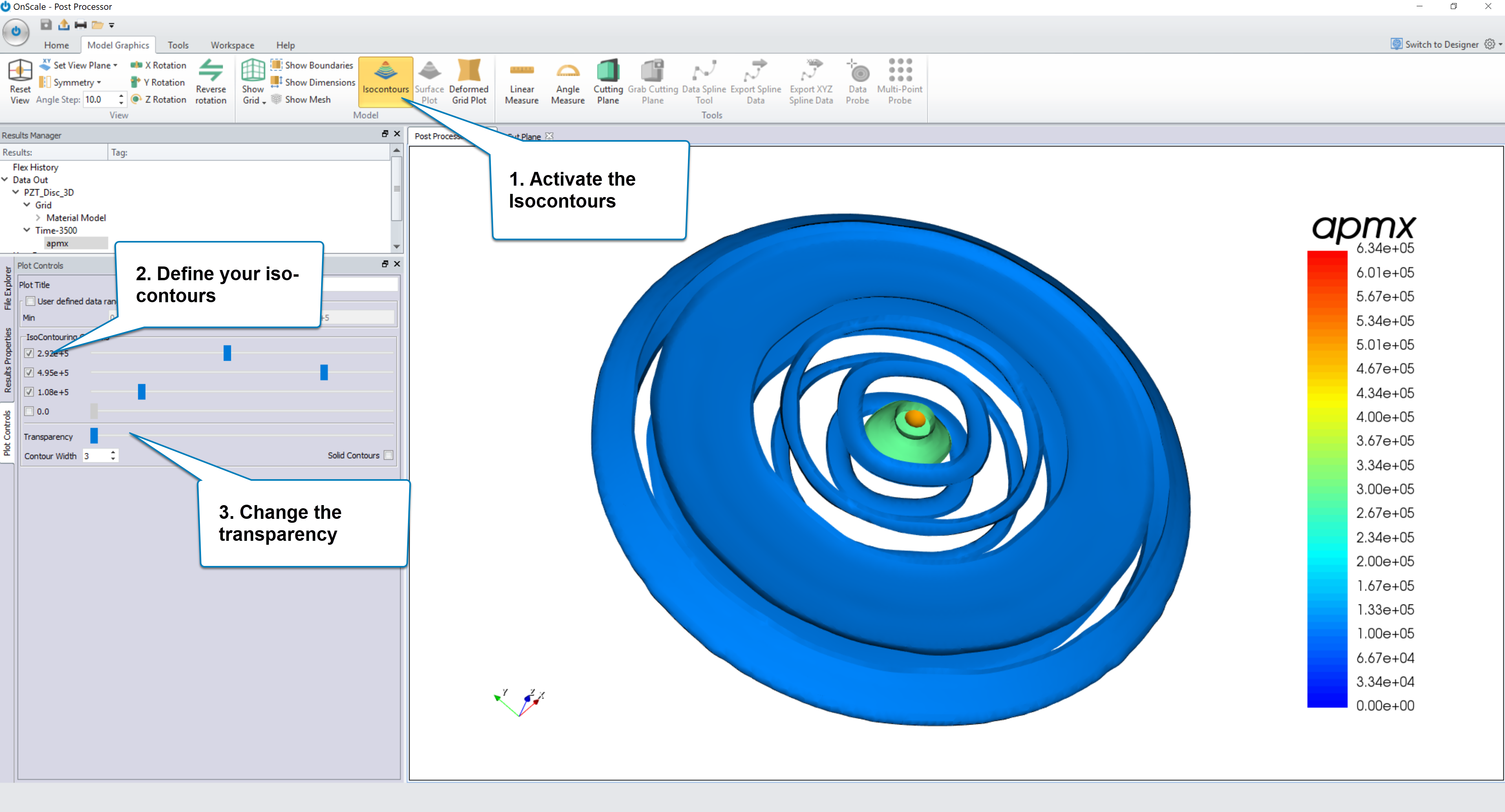
Iso-contours are used when you want to plot only a certain value of your results in the whole model and look at the spatial distribution of that value.

i.e.: You want to know where in your model the maximum acoustic pressure is equal to 292 MPa.

Here’s how you do it:

1. Activate the Iso-contours
2. Define the value of your iso-contours
3. Change the transparency to vizualise better

1.2 Surface Plot

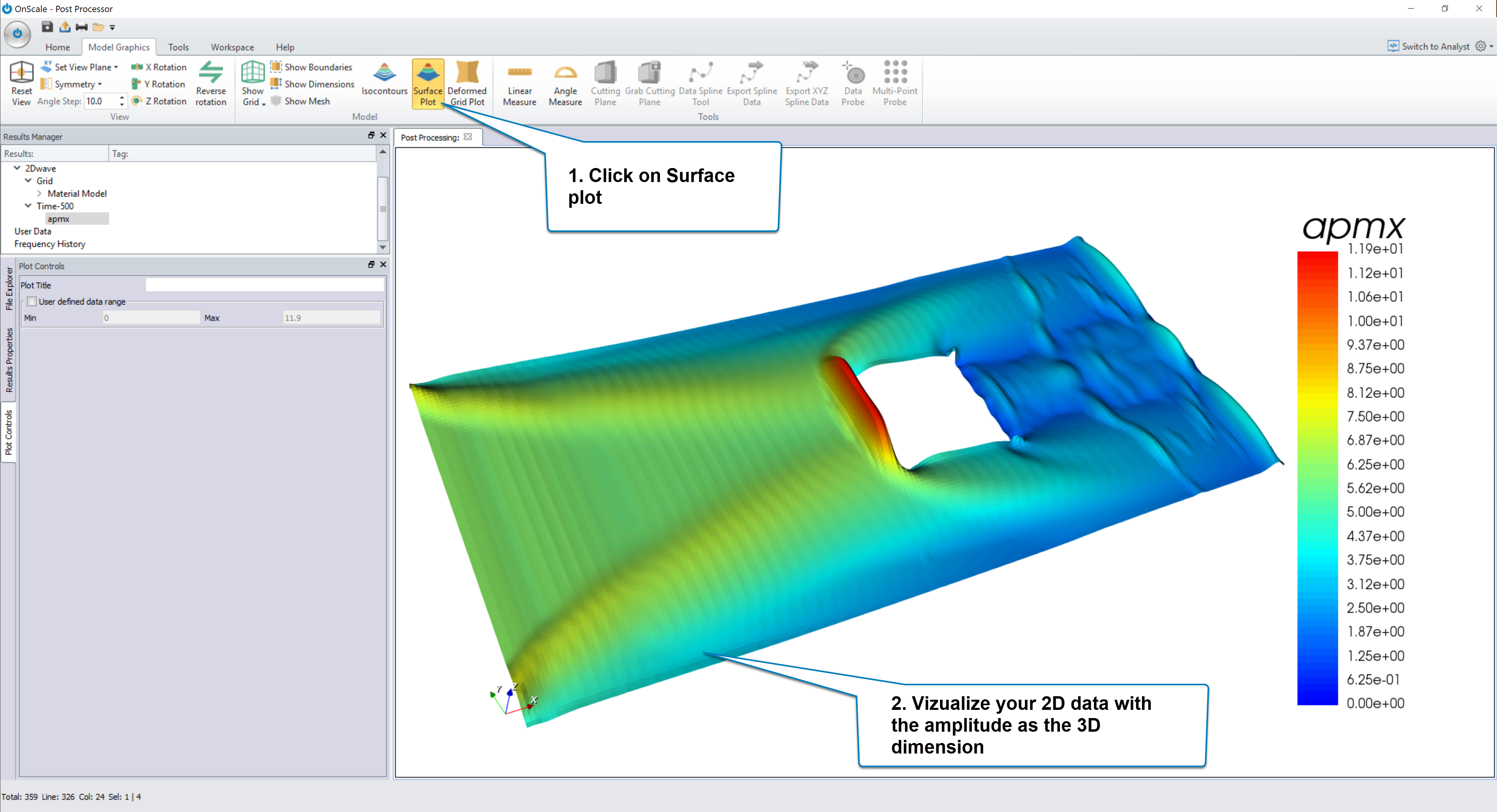
The surface plot is used to apply a visual deformation to a 2D Plane Strain (PSTN) model to represent amplitudes in terms of a 3D height. This is applied to requested quantities like pressure and stress etc.

Here’s how you do it:

1. Click on surface plot
2. Vizualize your 2D data with the amplitude as the 3rd dimension

1.3 Deformed Grid Plot

The deformed grid plot applies a visual deformation to a displacement snapshot. All components of displacement must be output for snapshot.

i.e. :When you generate your snapshot, make sure that the displacement data are inside the snapshot, then you will be able to vizualize the deformed shape of your model.

1.4 Cutting Plane

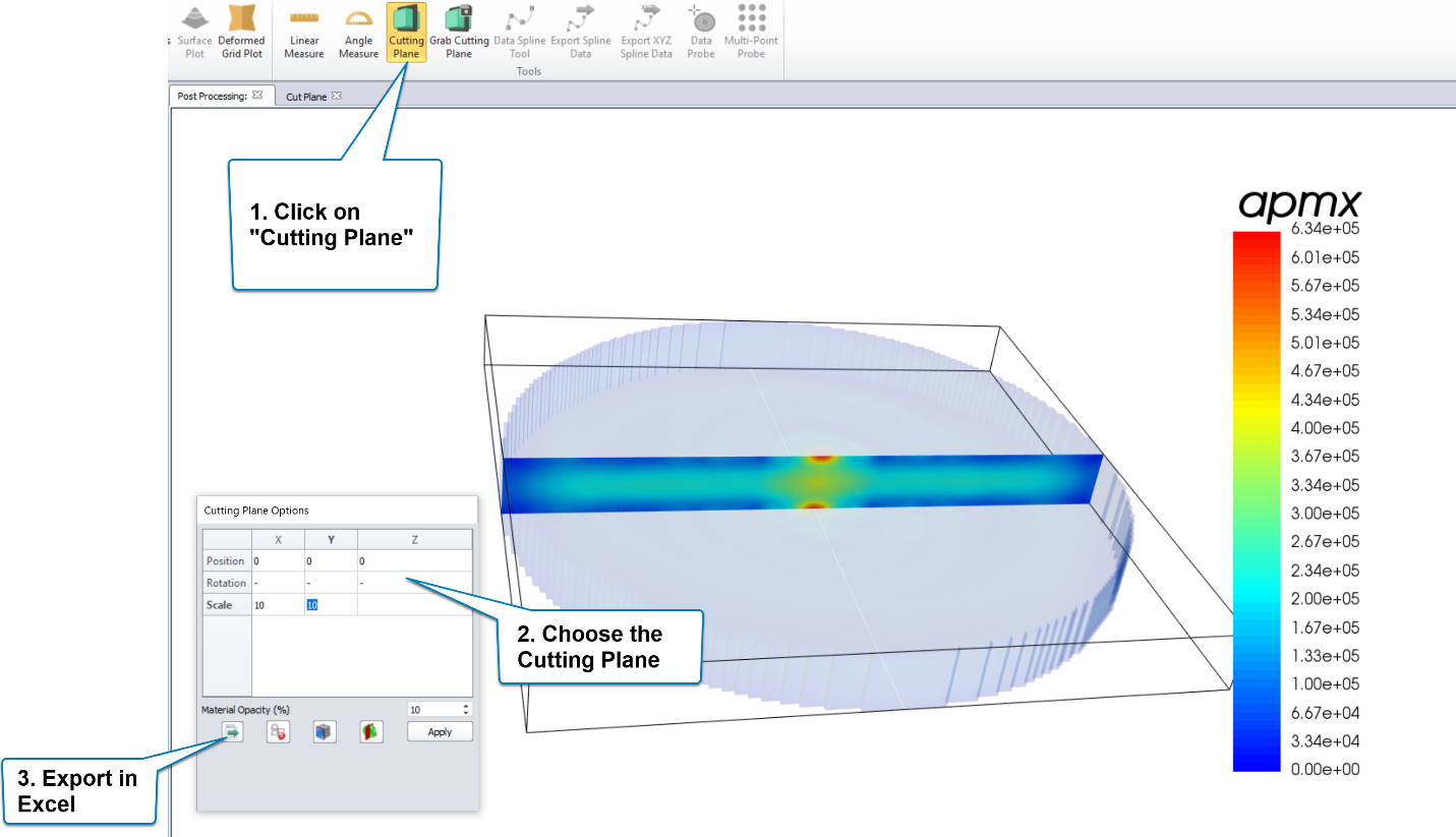
Like the name indicates, the cutting plane allows you to “cut” a slice of data from your 3D model.

Here’s how to use it:

1. Click on “Cutting Plane”
2. Choose the Cutting Plane Corrdinates (Or move the plane by dragging the arrow on the screen)
3. (Optional) Export the plane data in Excel to look at the results more conveniently

1.5 Grab Cutting Plane

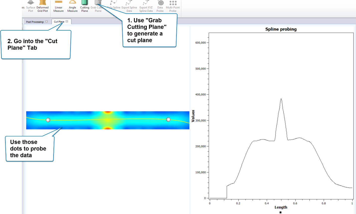
This function works in conjunction with the cutting plane. You can use it to extract the selected plane into its own tab to analyze it in more details.

What I find cool is that you can drag the dots on the plane to display a curve of the data going though a spline curve.

Here’s how to use this function:

1. Use “Grab Cutting Plane” to generate a cut plane.
2. Click on the “Cut Plane” tab
3. Move the dots to probe the data and display those data in the window on the right

1.6 Export XYZ Spline Data

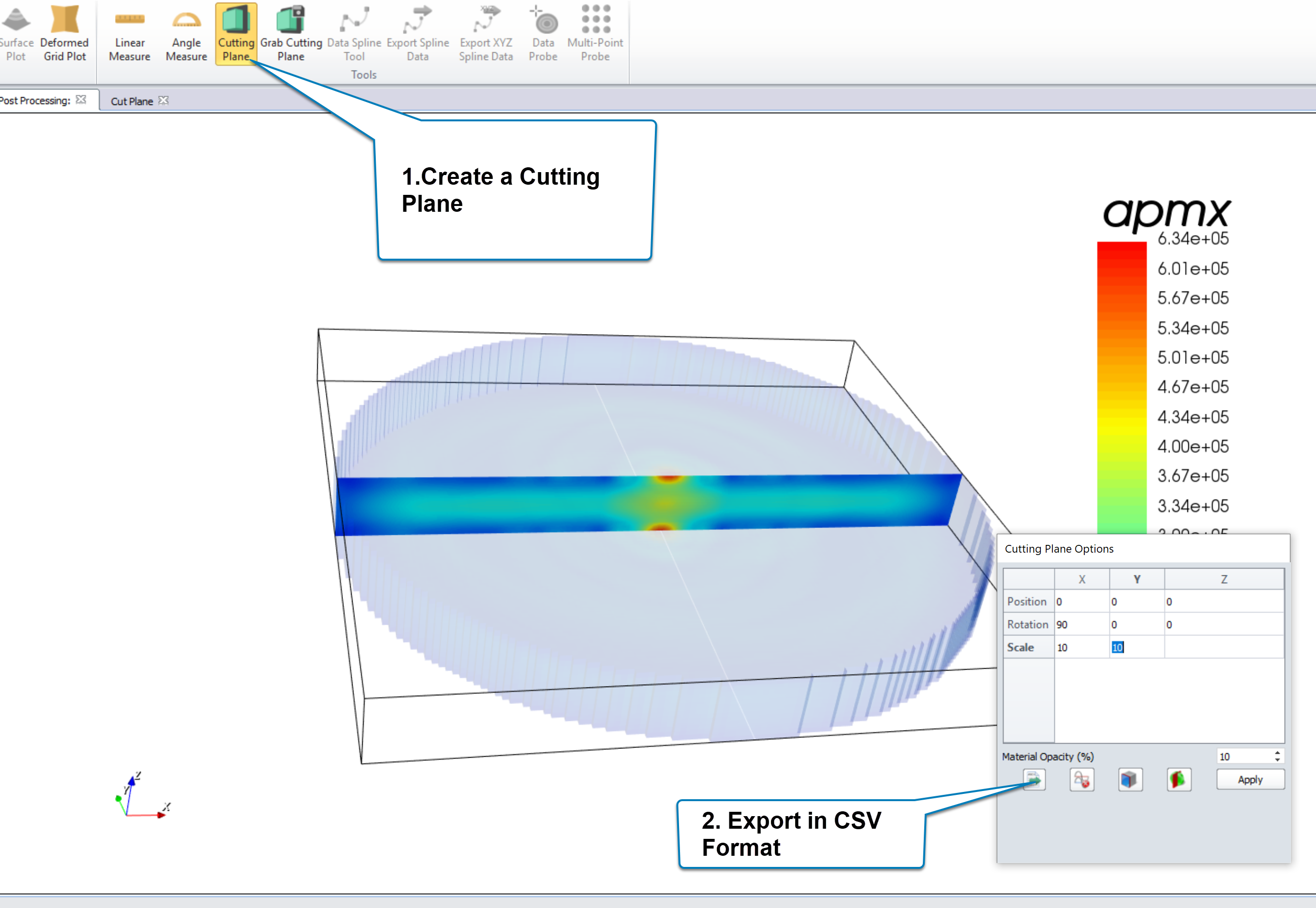
It is pretty easy to export results in Excel for further post-processing.

Just do the following:

1. Create a Cutting Plane
2. Export in CSV

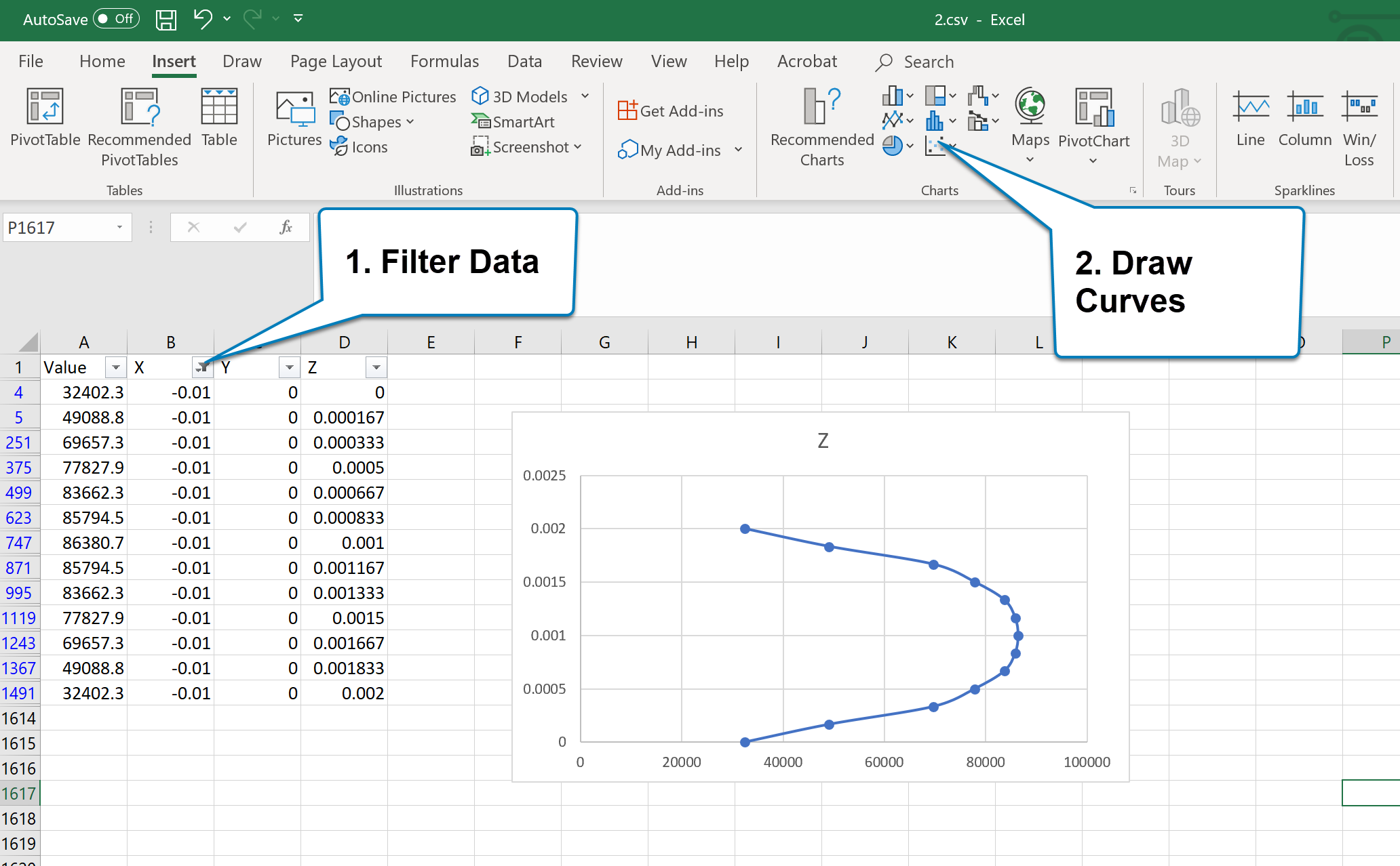
Post-processing in Excel can be as simple as:

1. Using filter to limit to choose only X coordinate for Example
2. Draw the curve you want

Ok, I think that now you start to understand better the kind of tools that you have in the post processor mode of OnScale.

Now, let’s talk about a more advanced part, which is the usage of custom scripts to post-process the data.

2- Post-processing using a Review script

OnScale has its own scripting language called “Symbol”. It is a scripting language based on FORTRAN that had been invented a long time ago when none of the actual more modern scripting language (like python) even existed.

The syntax isn’t very difficult to understand once you have seen a few examples (There are plenty of examples on OnScale support website)

Ok, let me give you an example:

Let’s suppose that you want to write a script which will export the value of the acoustic pressure at a certain position of your model and print out that value into a text file.

I think that you see the advantage of writing such a script… it’s a pain to write the first time, but once it’s done, it’s done and every time you re-calculate your model, you can just run that script and get it to do whatever you want just in one click :-)

The general way to write and execute Review Scripts is the following:

1. Create a new text window in OnScale Analyst mode and save it under the “*.revinp” format
2. Start to write your script in it, save and execute

Now, more specifically, how to tackle the example that I mentioned previously?

Here’s what we need to do:

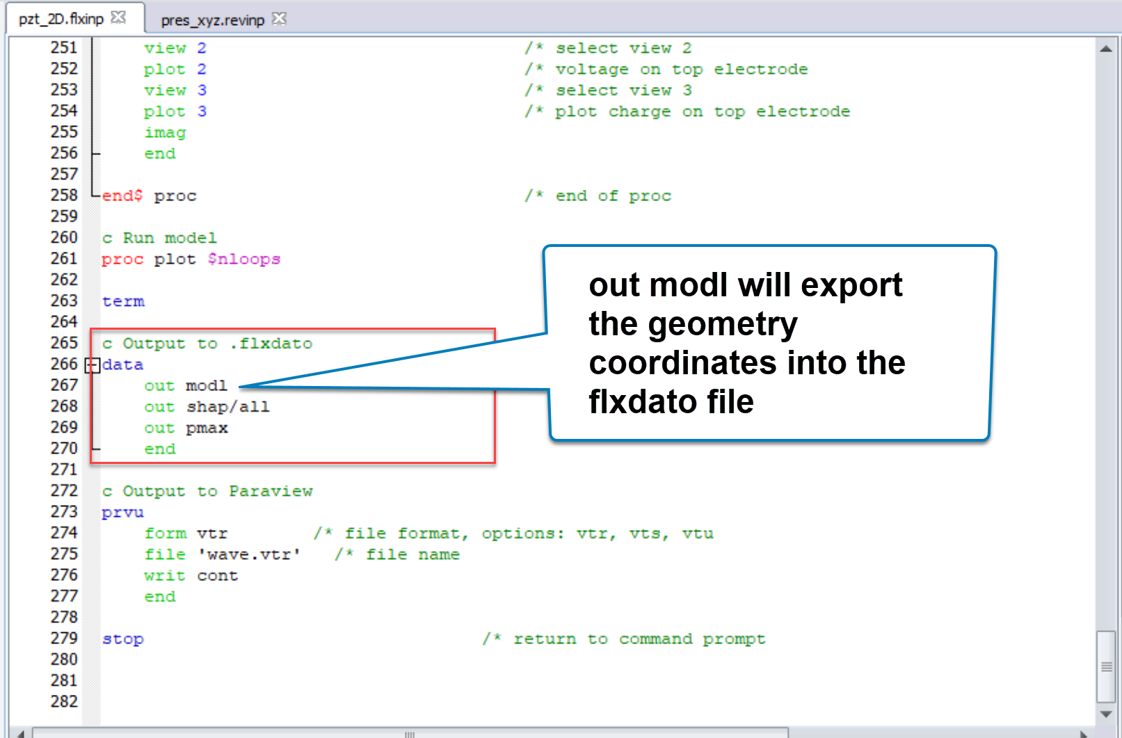
1. Find a way to export model geometry data (coordinates and nodes) into your “*.flxdato” output data file
2. Read this data file in your review script
3. Declare some variables defining the position where you want to obtain the pressure. Let’s call this position (px,py)
4. Get the nodal coordinates (i,j) of the nodes the closest to that position that you defined
5. Get the value of the pressure at that node and save it into a variable pval
6. Output that pval value into a formatted string and into a text file

The solution:

To export model geometry data (coordinates and nodes) into your “*.flxdato” output data file, you need to add data out modl in the data command of the main “*.flxinp” file of your model (and then run again your simulation)

Once you did that, write the appropriate Review script to execute all the step I mentioned previously:

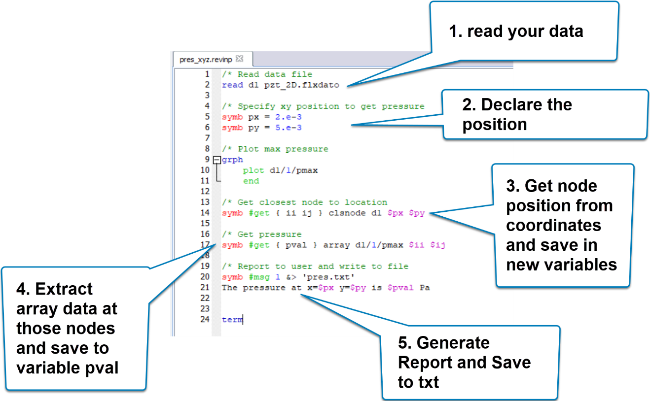
I give you the script… lucky you ;-)

Just copy, paste and run

/* Read data file
read d1 pzt_2D.flxdato

/* Specify xy position to get pressure
symb px = 2.e-3
symb py = 5.e-3

/* Plot max pressure
grph
	plot d1/1/pmax
	end

/* Get closest node to location
symb #get { ii ij } clsnode d1 $px $py

/* Get pressure
symb #get { pval } array d1/1/pmax $ii $ij

/* Report to user and write to file
symb #msg 1 &> 'pres.txt'
The pressure at x=$px y=$py is $pval Pa

term

Now enjoy your wonderful generated text file:

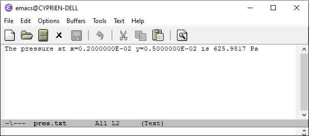
Of course, this is just a glimpse of what you can do with Review… with a little of imagination (and experience) you can do almost everything.

3- Post-processing using a Python (Or Matlab) Script

Even if you can do a lot with Review, you may still want to use a software that you are more familiar with to post-process your data.

Well… it’s actually possible ;-)

The first thing you need to do is to add the following code to your data command to save the results in matlab format

 

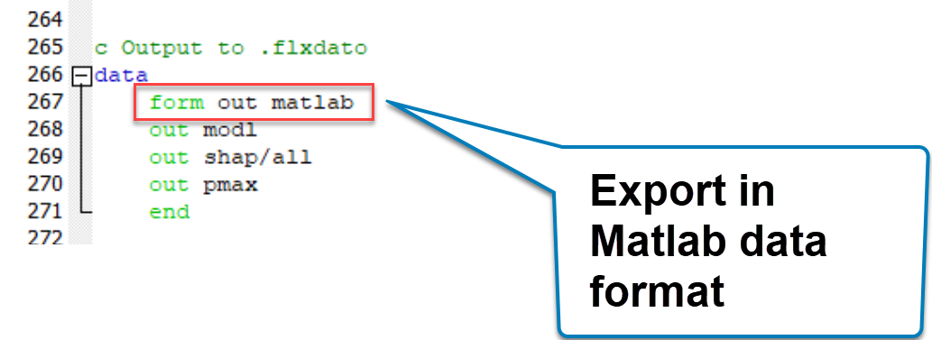
Once you did that, run again your simulation, and you will observe that your data will now be saved into a matlab readable format that you can directly open in Matlab!

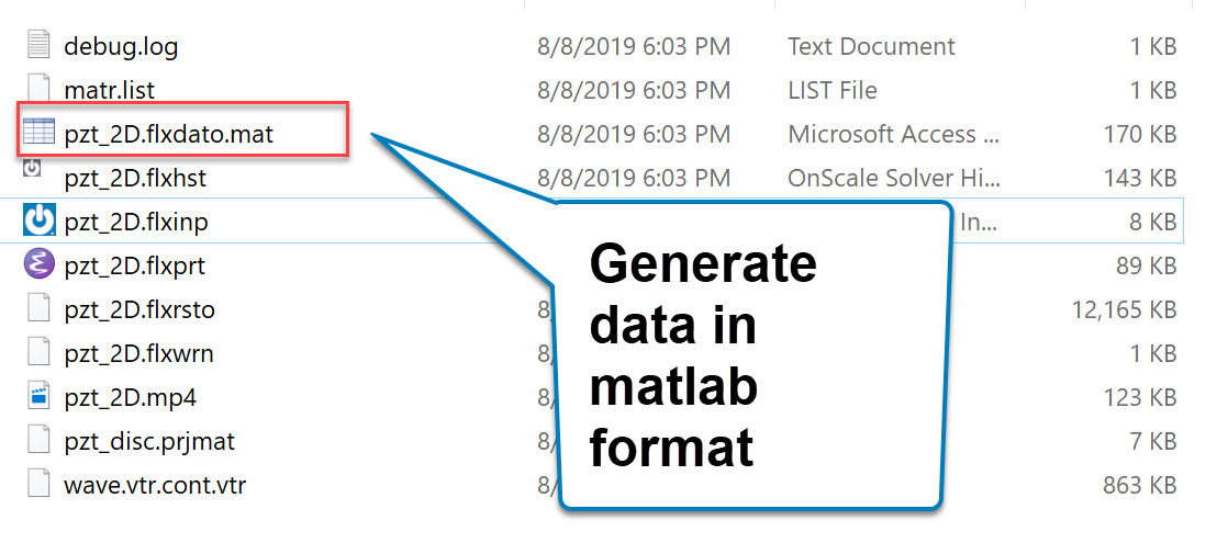
Now you can open it in Matlab and do whatever you want with it ;-)

How about Python?

Well, the good thing about having a matlab format file is that this file is also readable with Python!

You will find here a link to the scipy cookbook where it is explained how to read mat file.

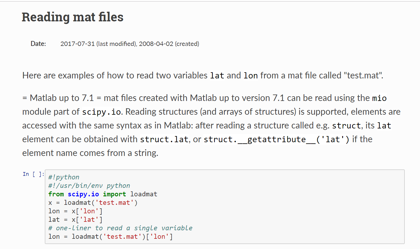
Here’s a simple example:

First, download this result file: pzt-simple-tuto-2d.mat

Let’s post-process with Python the data included in the apmx array (maximum acoustic pressure)

This is the apmx array vizualized in OnScale Post-process:

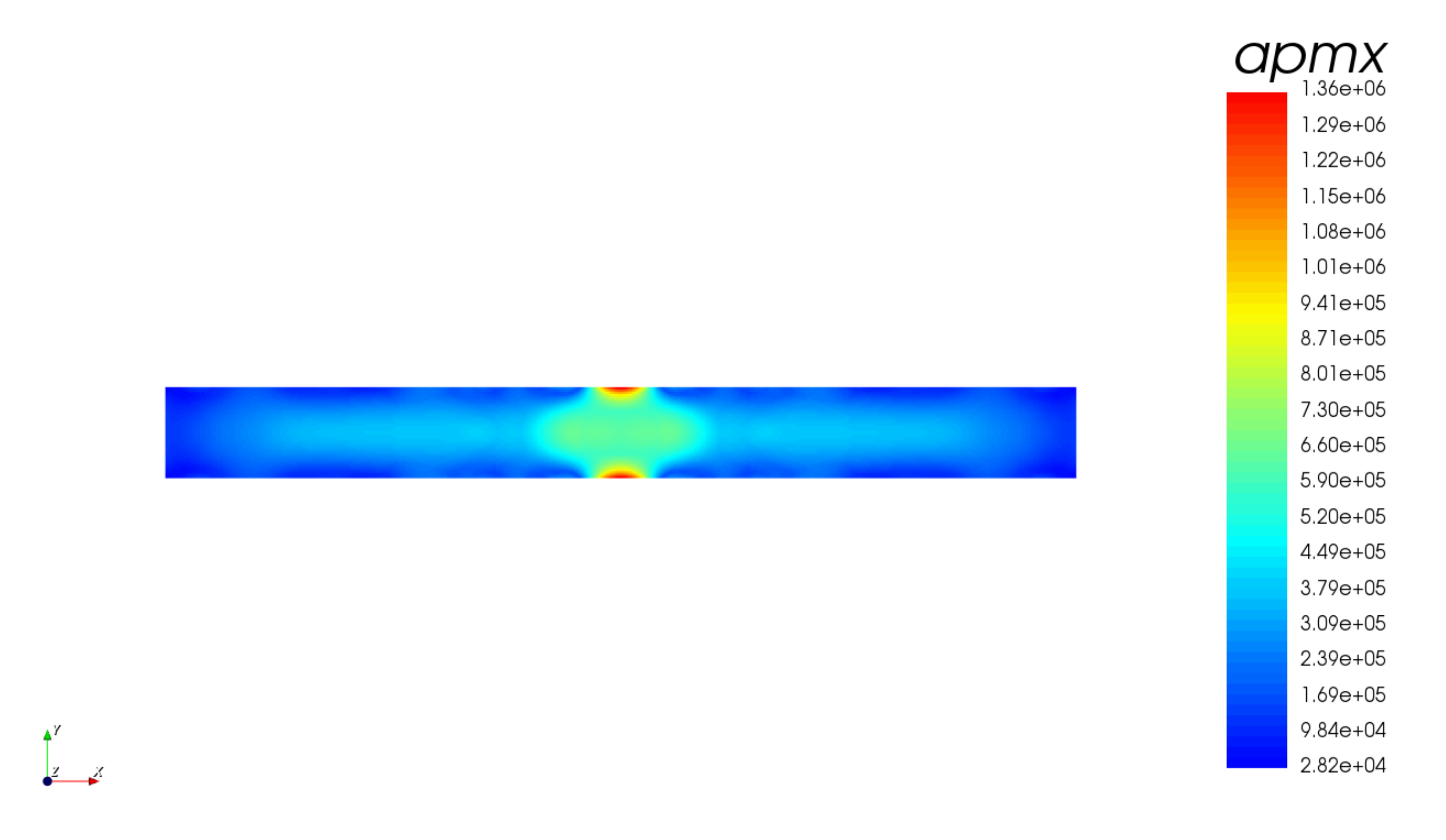
And here is a python script which does the following:

• Read in the data from the pzt-simple-tuto-2d.mat file
• Use the scipy loadmat function to load it into a variable called x
• Find the node i which corresponds to a certain xval coordinate
• Plot the resulting array

The Script

#!/usr/bin/python
import numpy as np
import matplotlib as ml
import matplotlib.pyplot as plt

from scipy.io import loadmat
x = loadmat('pzt-simple-tuto-2d.mat')

#Check the keys of the x array
print(x.keys())

#Extract the x and y coordinates
xcrd = x['d1_0006160_xcrd']

#Find the i value corresponding to a certain xval and save it to ival
xval = 150e-05

sampling = round(float(xcrd[2]-xcrd[1]),8)

for i in range(len(xcrd)):
    if(xval > xcrd[i]-sampling and xval < xcrd[i]+sampling):
        ival = i
print(ival)

#Plot the aprs in function of ival
plt.plot(x['d1_0006160_apmx'][ival])
plt.savefig('d1_0006160_apmx.png')

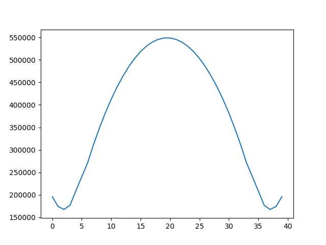
This python script postprocess the results and extract a curve at a position x = 150e-05

This is the resulting curve:

Note: You will need to install Python as well as numpy, matplotlib and scipy modules to follow this tutorial

4- Post-processing using Paraview

If you have used other open source software in the past, you probably heard about Paraview which is an open-source Generalist post-process.

You can download it here

Paraview is very powerful… but somewhat difficult to use if this is the first time you use it!

I made a video to explain this part:

This is a quick video to teach you:

• How to export your onscale results in paraview vtu format
• How to open that in paraview and apply a simple filter

I’ll show you here as an example how to apply the “Cell Data to Node Data” filter to view OnScale stress results at the nodes.

 

---

Ok, that’s about it for today! …. Lot of Stuff to unpack here

If you like this article, help me by share it on your preferred social network or send it to your colleagues, that would make my day :)

–Cyprien

 

 

 

 

Any idea for the next tutorial you would like to see?

Post a comment and let me know!