A Story about FEA principles

When you work with FEA for a long time, it's only natural to wonder about the initial physical principles behind the software we use every day...

It's nice to have a graphical interface with buttons, ways to draw and make calculations... but  where does all of that comes from and what are the physical equations used to perform those calculations?

The truth is that's a tricky topic... quite complex to grasp in its entirety... and full of differential equations and theorems which are gathering dust in mathematical books for ages.

One of my friend, who is also an engineer with a very solid background, decided to spend some time to simplify and turn the FEA principles into a story easy to understand.... Nice, right?

Here's a quick description of the Author of the article 

The story that follows will teach you in a simple way the principles of finite element analysis. Here's what you will get from it:

• You will understand which principles of mechanics are used to build the FEA Theory
• How to describe those principles with equations
• How to transform those equations into algorithms
• How to use those algorithms to solve practical mechanical engineering problems

Let's start our voyage to the FEA wonderland... ;-)

Note: If you want to download it in PDF to read it later, I will put some links to download inside the article.

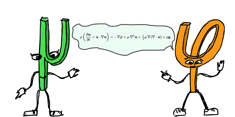
Mr Phi is a bright physician but he is trying to solve really tough equations. Among them, you can think about Navier-Stokes equation (no general solution so far) or the static continuum equation: 

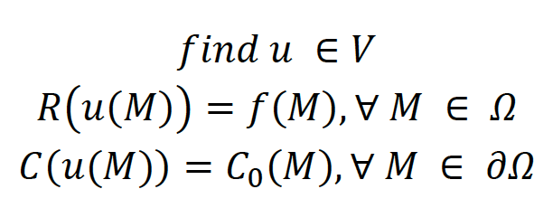
Not to ease his task, he is trying to solve them on very complex geometries and boundary conditions: 

Wow, this looks like a world of pain. So, Mr Phi goes to Mr Mu for help. Even to Mr Mu, these problems are very complex. But Mr Mu has the power of abstraction of Maths with him. He has the ability to gather a whole lot of problems in a generic format for which he can find out very helpful theorems. 

More specifically, Mr Mu informs Mr Phi that if he can adapt his problems to the world of linear Algebra, a lot of tools could be called. 

Mr Phi: “Hey Mr Mu, what do you mean by adapting to linear algebra. I mean, I have studied it at school, but could you be more specific?” 

Mr Mu: “Alright buddy, I see you are willing to be more accurate, so let’s go” 

Firstly, let’s characterize what you are trying to find. Usually, you are talking about a continuous field defined in 3D space, and sometimes you want to see its evolution in time (and sometimes the steady state is ok for you). To begin with, let’s forget about time for now. All I see right now is that you are trying to solve: 

• Variables = M points in a domain named Ω, described by coordinates x, y, z, 
• Field = usually a scalar function u(x,y,z,t) like temperature or a vectorial function u(x,y,z) like displacement. We can then decompose u in scalar functions ux, uy, uz. 
• This field must be solution of an equation R(u)=f for all points in Ω 
• You often have specific values of u or its derivatives on the edges of Ω that we call ∂Ω. We call these specific values the boundary conditions. We can gather them in a set of boundary conditions that we call C(u(M))

# R is an operator that transforms u in a mix of u, its derivates, multiplied and summed with other functions. Something nasty I don’t wanna know about, that we will call a “differential operator” 

# f is another function of x,y,z. Something nasty as well, but without u in it. 

More properly written: 

• R is a differential operator on the space of u functions 
• u are functions defined on Ω, that are enough differentiable to stand the R operator. We will call V the space of these functions 
• f is a function of same type as u (either vector or scalar) 
• C is an operator on the space of u function 
• C0 is a set field on the edge of Ω

Mr Phi: “Fair enough, I bring you precise equations about how the world goes round, and all you want from me is R(u)=L ! Thanks for respecting my science!” 

Mr Mu: “What I am trying to do my friend is to conceptualize your problem. It is so complex that I am first trying to see it from helicopter view. It is too early to go deep into the specific terms of each equation” 

“Let me go on and tell you how you could fit your problem to the linear algebra” 

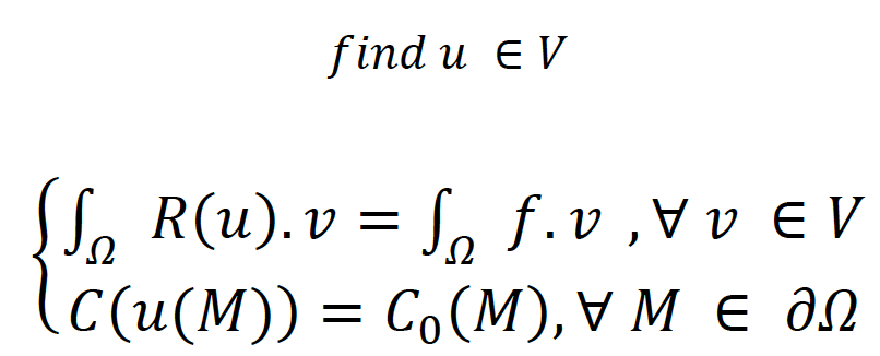
Step 1: Let’s multiply everything with a random v function and integer it on Ω

The problem now looks like this: 

Mr Phi: “Why did you do that?” 

Mr Mu: “You will see later my friend. There are several interests: 

• If R(u)=f was a vectorial equation, we have now a scalar equation 
• If I choose v smartly, I will be able to simplify my equations when needed 
• I can prove that this formulation is equivalent to the initial one 
• I am trying to create a scalar product here, wait a little more please” 

Key point : equivalence of weak formulation and initial formulation: 

Step 2: Get to bilinear and linear forms

Mr Phi: “This is where you rework your physical equations for me” 

# To do so, we will use several tools and assumptions: 

• Integration by parts 
• Green integration formulas 
• Assume that some coefficients in your equations are constant

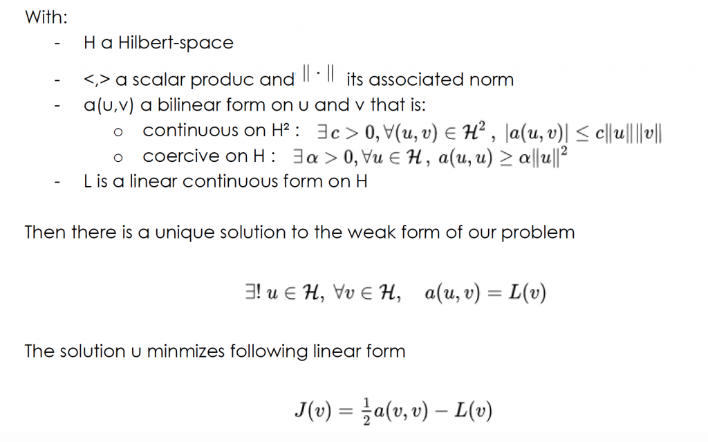
# In the end, your problem should have the formal presentation like this: 

• a is a bilinear form on functions in V 
• a satisfies several mathematical conditions (coercive, continuous) 
• L is a linear form on functions in V 
• The information of boundary conditions has been included in the weak form, through integration by parts and Green formulas

# For a given problem, you can find several weak formulations. Some of them are well documented and “standard”. For example, you can google “weak formulation elliptic problem” or “weak formulation Dirichlet problem” and see that many physical equations can fit this format. 

Here's the Lax-Milgram Theorem:

Mr Phi: “You tell me there is an answer, great! I am now awaiting this answer!” 

Mr Mu: “I understand. Even in this linear algebra world, I cannot easily give you an answer, because the vector space of acceptable solutions is of infinite dimension. However, we have made a great progress.” 

Mr Mu: “We will now try to approach your solution on a finite dimension vector space of functions” 

Do not hesitate to dig into Lax-Milgram Theorem on Google. It is elegant maths ! 

An element is a domain of 1D, 2D or 3D space in and/or on which you have nodes. The idea is that we calculate field values (nodal values) on nodes and then estimate field values anywhere inside the element with the nodal values.

But for now, let’s just stick to the basics.

Element = domain (in 1D,2D or 3D space) + nodes

Here are examples of elements

There are a lot of types of elements, but these are the usual ones.

​3.2 Nodal values and interpolation

Concept on a basic example:

Let’s say that you have a scalar field u defined on a dimension 1 space, u(x) for x in I=[0;10]. You don’t know u(x) on the whole I interval, but only on specific x values, let’s say 0,1,2,3..,10. Said in the FEA language, you only know 11 nodal values u0, u1, …, u10

You also know that u is continuous. Can you think of a method to shoot approximate values on any x, knowing only the nodal values? In other words, how to connect the dots?

Well, the basic thought is that,

• u(2.5) is somewhere between u(2) and u(3).
• u(2.1) is closer to u(2) than to u(3)

Warning : this kind of belief is adventurous and sometimes very wrong. This is why FEA must always be applied with a good physician sense.

So, in action, you can imagine several interpolations, i.e. several ways to connect the dots :

Linear interpolation (with straight lines)

Polynomial interpolation (with pieces of polynoms)

Example of interpolation error, with Lagrangian polynoms

More formalism on linear interpolation:

There are many methods to interpolate (connect dots). We will not see all of them here, please feel free to google the topic to learn more about that.

For now, we will formalize more cleanly the linear interpolation = connecting dots with straight lines in 1D space. Let’s do it on our [0,10] interval with 11 nodes 0,1..10

# First of all, we define 11 “hat functions” as φi centered on each node. These functions φi worth 1 on the node i, and reach 0 on surrounding nodes i+1 and i-1 and then stick to  on the rest of the domain.

 # We also already have our nodal values ui

# With all of that we then write the formal expression :

Uh is now a function of the subspace Vh = the sub-space defined by linear combinations of φi functions.

The application of such a formal expression generates a curve like this (ui are the red dots) :

Linear interpolation (with straight lines) = sum(ui*φi)

Hint : FEA softwares often use this basic linear interpolation. Where the u field seems to vary very quickly, it will beup to the user to refine the mesh (number of dots) around the critical area to compensate the error due to linear interpolation.

This interpolation in 2D or 3D is a bit uglier to write, but the principle is really the same. The interpolation functions (also named test functions) worth 1 on their associated node and must reach 0 on the borders that are not connected to this node (border = edge, node or face)

Here is a visual image of the hat function in 2D :

Hat function for node i on a 2D space

3.3 Problem in the finite dimension vector space

Let’s remember our general weak formulation

In §2.2, V was the vector space of acceptable functions with regards to continuity, differentiation and boundary conditions. V is of infinite dimension.

What if we replace V by Vh, the vector space of functions that are a combination of test functions :

Vh is :

• a finite dimension vector space, and a sub-space of V
• The φi hat functions are a base of Vh

Mr Mu: “We have now a sub-problem of our initial problem. It is in finite dimension vector space à we can decompose the function on a base with a scalar product + use matrixes à computers like matrixes!”

In our linearized world, the weak formulation can be written as following when restricted to Vh :

With i from 0 to 10, and choosing φi as test functions, we can easily get a matrix of 11 equations of the 11 variables ui à and the computer solves it!

Replacing V with a sub-space Vh is the Galerking method

​

​3.4 Why would the FEM solution be a good a good approximation ?

Mr Phi : “Wow my friend, you really have some skills in your elegant way! But I have several doubts on your method that I would like to discuss…”

• How close is uh from u?
• You asked me to linearize my physical equation earlier: what error have I made doing so?

Mr Mu : “Well, I am going to answer your first question. The process we have just shown in this paper is the solving of linear static problem or linear steady state problem. The second one will be discussed in another paper, as there is a complementary method for non-linear static/steady state problems. I will tell you now a few words on the error between uh and u.”

Céa’s Lemma:

This mathematical theorem will help us estimate the error between u and uh. Let’s remember our weak formulation problem.

We have defined the problem on V with physics, and computed a solution on the finite dimension subspace Vh

Let’s also remember our operators on V :

• <,> the scalar product with which we established the necessary continuity and coercivity properties on a and L
•   its associated norm

We can bind our solutions u and uh with the following relationship, which is Céa’s lemma :

What does it mean?

This means that, up to the C factor, in the meaning of the   norm, uh is the best approximation of u on Vh

Mr Phi: “Great! But are this C-factor and this norm a good way to judge the quality of my approximation?”

Mr Mu: “Not always! Please remember that you always need to keep your good physician spirit. Some important remarks:

# Céa’s lemma tells you that you have the best approximation on an overall measure which is the norm. But uh can be very close to u somewhere and pretty far from u somewhere else, and eventually close with regards to the overall norm.

# You also have the best approximation on Vh. You can have better approximations on other sub-spaces, which means:

• Other meshes (especially when you refine the high variation zones)
• Other element types and test functions (quadratic elements for example)

Experience will do the rest !

# You can prove that if the mesh tends to infinite refinement, uh tends to u. This means that the more you refine, the more you get close to the real solution. Practically, when you see that refining your mesh doesn’t change the results, you can think that you have a good approximation.

​4. In action : the complete elliptic Dirichlet case

​4.1 Presentation and weak formulation

We want to solve the following classical problem :

​

Weak formulation :

We have discovered that this problem is equivalent to the following one

After integration by parts on v we get :

Let’s define, to ease the writing, the following bilinear form on V :

And the following scalar product :

The linear form of our theoretical approach is :

​We will divide our domain into 5 equidistant elements (6 nodes) :

For each node i we define:

• ui the nodal value of u (unknown)
• φi the hat function centered on the node i
• fi the nodal values of f (known values)

If u is replaced by a solution on Vh space like this

We choose on purpose 6 test functions for our vi à we will get 6 equations for j from 0 to 5 like this :

We can already calculate the famous a bilinear form for tests functions :

and pour them in a matrix. φi’ equals either 0, +10 or -10 depending on where we are around the I node. I let you do the maths, but the a bilinear form put in a matrix look like this :

We can already calculate the base scalar products and put the results in a vector :

In our vector sub-space Vh, with the φi as a base, uh function is a vector

The general writing of the discretized problem becomes :

Therefore, we will just ask the computer to solve the following system :

# I hope this step by step paper helped you get the spirit of FEA theory. Of course, we have been fast on the very formal maths but it was not the point. The point was that now, if you want to dive deeper in a theoretical course, you will find it easier. For that, please let me know if the mission is accomplished!

# Mr Phi is now very happy since he has a good method to solve linear static or steady state problems. However, he already wants more! Indeed, he has trouble in the following cases:

• When the physical equations become hard to linearize. Examples : large strains, non-linear constitutive equations, etc.
• When time comes at play

# Also, we brutally said in §4.4 “we will ask the computer to solve the matrix equation”. How does the computer do that? How do algorithms work? This deserves specific articles as well.

# So Mr Mu will return for further chapters !

Cédric Khayat

———–

That’s all basically for this article… and that's a LOT of knowledge to unpack ;-)

Take all the time you need to read and if you want to share your ideas, please just write what you think in the comments and let me know

Thank you so much for reading, I hope you learned a lot!

–Cyprien