[Salome CFD Tutorial 1] Simulating a simple 2D channel flow from A to Z with Code_Saturne

Important Note: There is newer version of this video now available here as Salome CFD/Code_Saturne has changed a bit since 2018. Most of what you will read here are still mostly relevant, but there are some changes in 1) The way to install Salome CFD 2) The Options and Menus in Code_Saturne

Here’s the link to the Salome CFD download page: Download Salome CFD

First tutorial I make on the open source CFD code Code_Saturne integrated into SalomeCFD!

In this video you will learn:

• How to install Salome CFD – How to model a simple channel (Geometry) in the Geom module of Salome CFD
• How to mesh and prepare it for CFD into Smesh
• How to post-process your results with Paravis to display the flow pressure and velocity AND how to draw a flow profile curve!

---

in today’s video tutorial we’ll talk about Salome CFD.

It’s the first video I’m doing about open source fluid dynamics with Salome CFD and Code Saturne, so I hope it will be very interesting!

Salome CFD is different than Salome Meca because it integrates Code_Saturne instead of Code_Aster

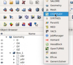
CFD study is the module that uses Code_Saturne in Salome CFD.

But how do you actually install Salome CFD ?

The way to install Salome CFD has changed since 2018. Check this article for the latest way to install Salome CFD:

Installing Salome CFD in 2022

Tutorial : 2D Simple Channel Flow

Let’s start the tutorial

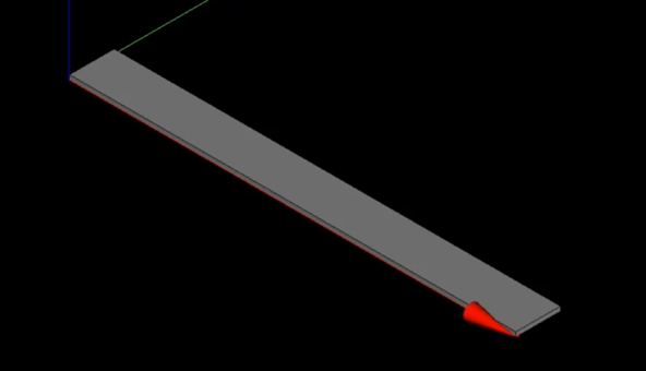
I will start with a very simple flow analysis of a simple 2D channel and the first thing I’ll do is to create the following geometry model:

Step 1- Creating the 2D Channel Geometry

let’s go into the geometry module in which I will build the model that I will use for this tutorial

For the sake of simplicity I will do a 2d analysis but you should know that you need still to

have a 3d model which will have only one layer of mesh in the z direction

(That’s how code Saturn works)

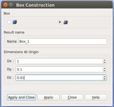
I need basically for this to build a simple box :

My model will be very simple it will have a length of :

• 1 in X Direction
• 1 in Y Direction
• 0.1 in Z Direction

So now I have a block and I have to think about what I need to do to set up the mesh and and make this model ready for simulation

Well I need to create the groups

Note that the groups are important as they define the areas where boundary conditions will be applied in Code_Saturne

Step 2- Creating the Geometry Groups

So let’s define the groups

The first type of groups to create in this type of model are « edge groups » which will help to define the size of the mesh in the next step.

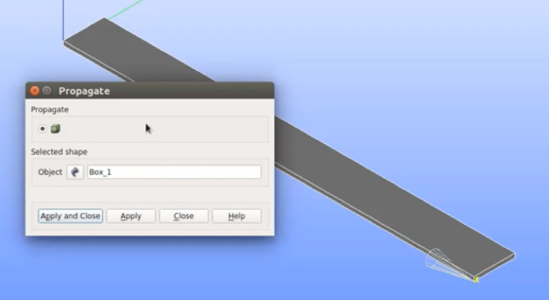
When the geometry is a block, there is a function Operations>Block>Propagate that can be used to generate automatically some edge groups corresponding to each coordinate direction.

This function here creates three set of edges which are in each of the directions and I will use those sets later to define the sub mesh and constrain the number of elements of my model

You can change the name of each group so it’s easier for you after to assign them to the right sub-mesh

Now that I have that let’s create the groups that I will use to assign the boundary condition of my CFD analysis.

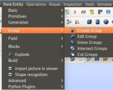
So let’s go in New entity>Group> Create group

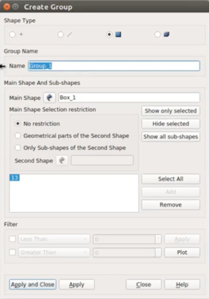
Select my geometry and select the shape type as « face »

Select the face where the inlet will be applied, click on « Add » and a number which represents the ID of the face will be added to the dialog box.

Then click on « Apply » and change the name to « Inlet »

Repeat the same operation to generate 4 groups of faces :

Inlet, Outlet, Walls and Symmetry

My geometry model is complete !

Step 3- Creating the Mesh

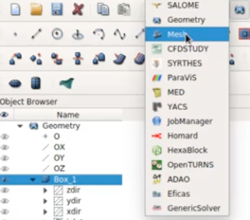
Now I will go to create the mesh so let’s jump to the mesh module and activate our geometry

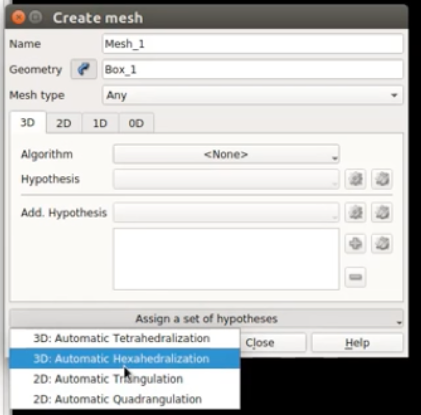
The first thing to do is just to add a new mesh set and then choose « 3D Automatic Hexahedralization » to simplify things a bit.

Once you did that, you will have some mesh, but there is still a problem… it will have the same number of elements on all its edges.

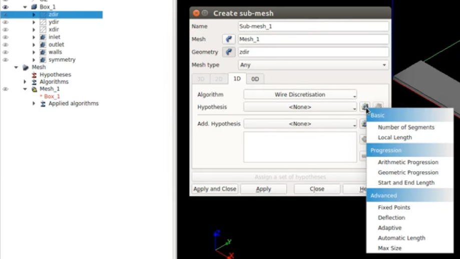
To specify how many elements you want, you have to use sub-mesh.

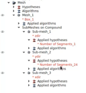
The only thing you have to do is to select one of the edge groups xdir, ydir or zdir and create a submesh which will define the number of elements to be used on that edge during meshing.

Let’s use the following numbers :

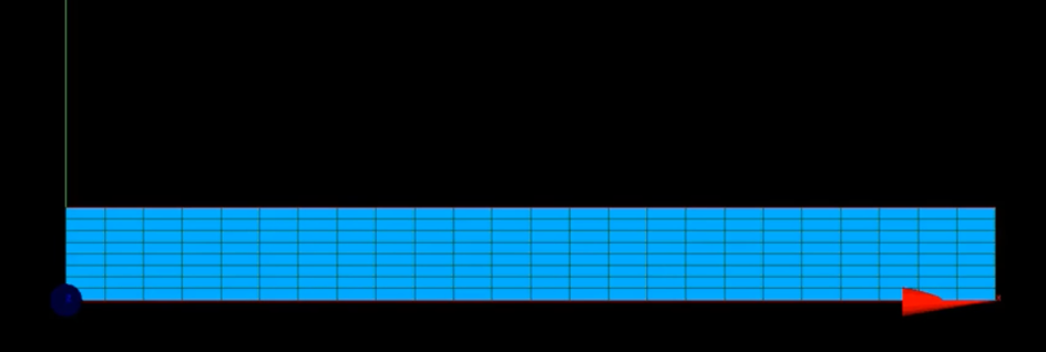
Y-direction : 8 elements

X-Direction : 24 elements

Z-Direction : 1 element (because we study a 2D CFD problem here)

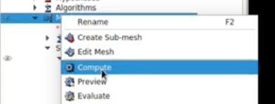
Once you defined all the submeshes, you can compute and get your mesh :

This is what you should get :

Step 4- Creating the Mesh Groups

Even if we created the geometry groups, we still need to create groups for the mesh

Why ?

Because the solver only look at the mesh… geometry groups are an help to generate mesh groups more easily.

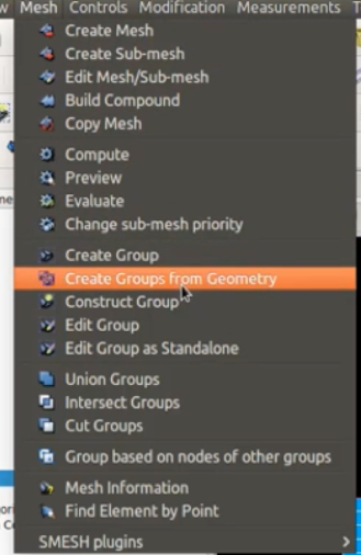
Fortunately, there is a function which can do that called « Create Groups from Geometry »

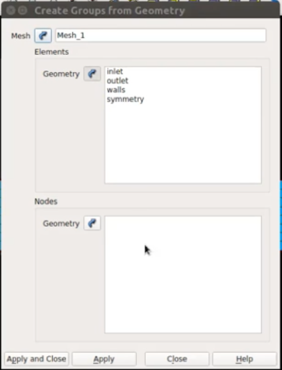
Use this function to generate the mesh groups :

This is what you should have in the Object Browser if you did it correctly :

Step 5- Defining the CFD Study

let’s go to the next step which is the definition of the parameters of the CFD study

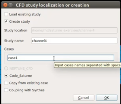
Once you open the module « CFD study », you have to create a new CFD case and save it.

Check « Create Study », choose where you will save it and then enter a study name and a case name, then click on OK.

Save the new study and you will see a set of new folders appearing in the object browser :

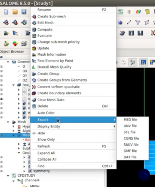
Important Step : You need to export manually the mesh set you created previously into the « MESH » folder.

For that, go back in the mesh module, select your mesh and in the menu choose « export in MED format »

Ok, now we are ready to set the CFD study !

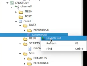
Go back to the CFD module, unfold the folder DATA from the object browser, right click on the « SaturneGUI » file and choose « Launch GUI »

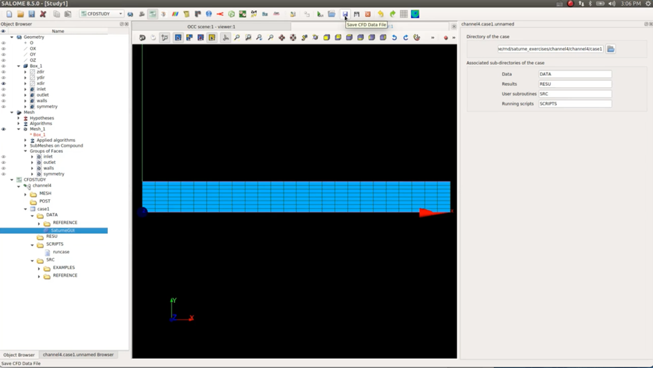
The GUI should open like that

Choose « Save CFD Data File » before doing anything else :

Note : If you don’t have this bar, you may have to go in the menu and activate it

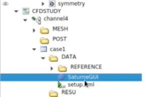
When you click on save, you see in the object browser that you have a  new XML file which appeared :

Everything you define in the Saturne GUI is also written in XML format into this file.

If you are not familiar with XML it’s a bit like HTML format but it allows to define your own tags so it’s used by the GUI interface to dialogue and exchange together the user input data.

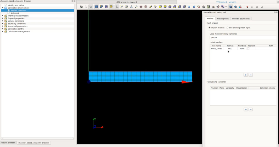
Next step is to define your mesh in « mesh selection » :

If I click on mesh selection you see that it automatically opens the folder MESH and now I have to click and add my mesh inside

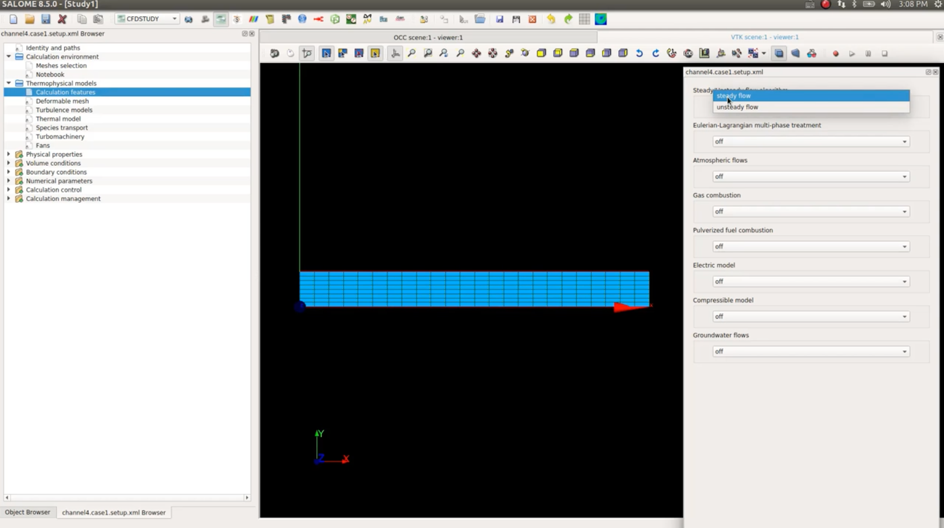
Now we have to go to « thermophysical model » and open « calculation features » where I can define the flow study as « steady-state »

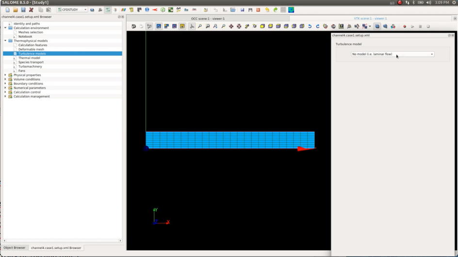
I won’t use any turbulence models as this will be a laminar flow so I’ll just set the turbulence model as « No model » :

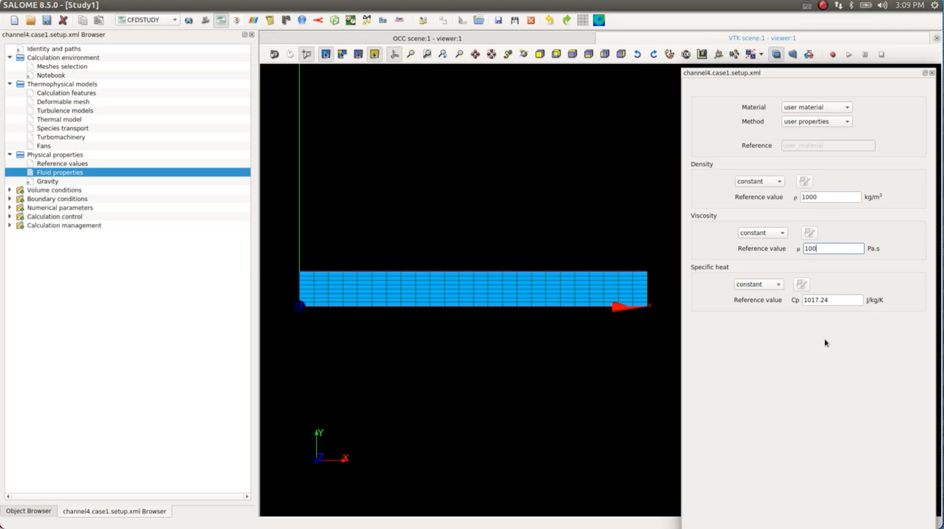
I need to define the properties of the fluid reference value so I’ll put density of 1000 and viscosity of 100

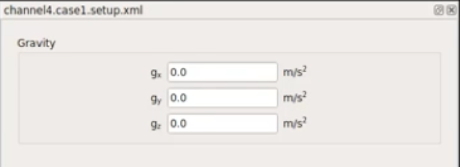
Gravity will be null in this case so but remember that if you want to consider the effect of gravity well you have to define it here:

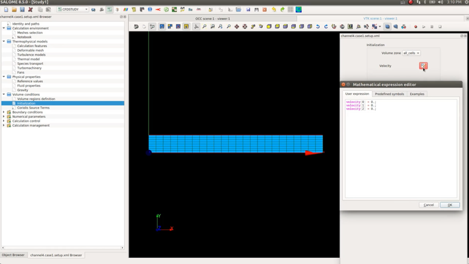
I’ll define now the initialization condition for the velocity as 0,0,0

(This is just an initialization condition, real velocity is defined on the « inlet » as a boundary condition)

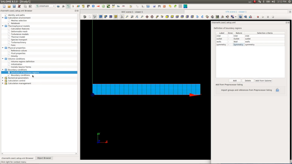
Now, let’s define the boundary regions as in the photo below. The name written in the « Selection Criteria » Tab should be the same as the name of the mesh groups defined previously.

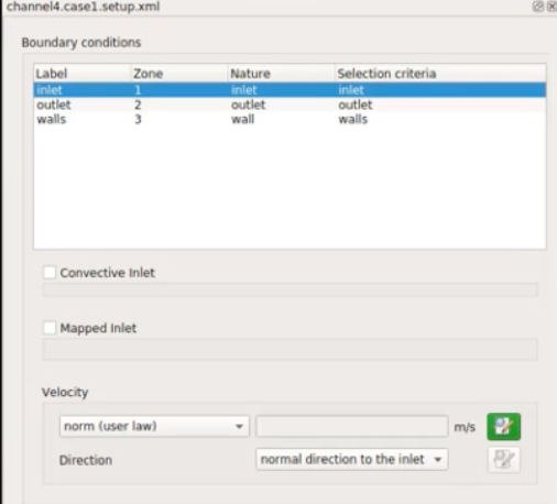
Then, go in the « boundary conditions » Tab and define the boundary conditions for the inlet, the outlet and the walls.

Here in this case, we only need to change the inlet to apply a velocity of 2/3 m.s-1

You can use and « User law » to define the velocity like a function

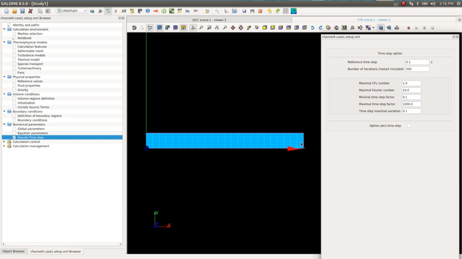
Now, we finally open the « Pseudo-Time Step » tab and we can define the number of iterations as 500.

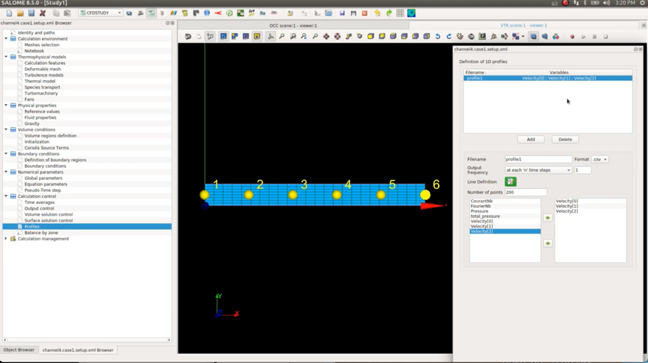
Let’s define now a few monitoring points at different positions which will help us to get the value of the velocity at each iteration and check the convergence status of the velocity at the same time.

Set the format to CSV to be able to open it in Paravis in the next post-processing phase.

In case you do not see any monitoring data output after computation, check that the export of monitoring data is activated in the « Volume Solution Control » Tab.

Let’s set now some velocity profiles, this will help us to get the velocity profiles exported in text format directly after computation :

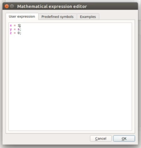
To select the place where the profile will be calculated, you can use the mathematical expression editor here and define the equation of the cut line.

Step 6- Compute the CFD study

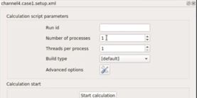
Once everything is set up, go in Calculation management> Prepare Batch Calculation, choose the number of processors you want to use and « Start the calculation ».

(In case you are using an installation of SalomeCFD generated for Scibian, you may have to change the version of openmpi installed on your computer… in this case try with 1 processor only first)

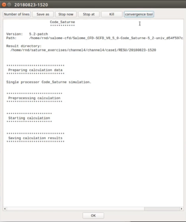
You will see a window like this one appearing :

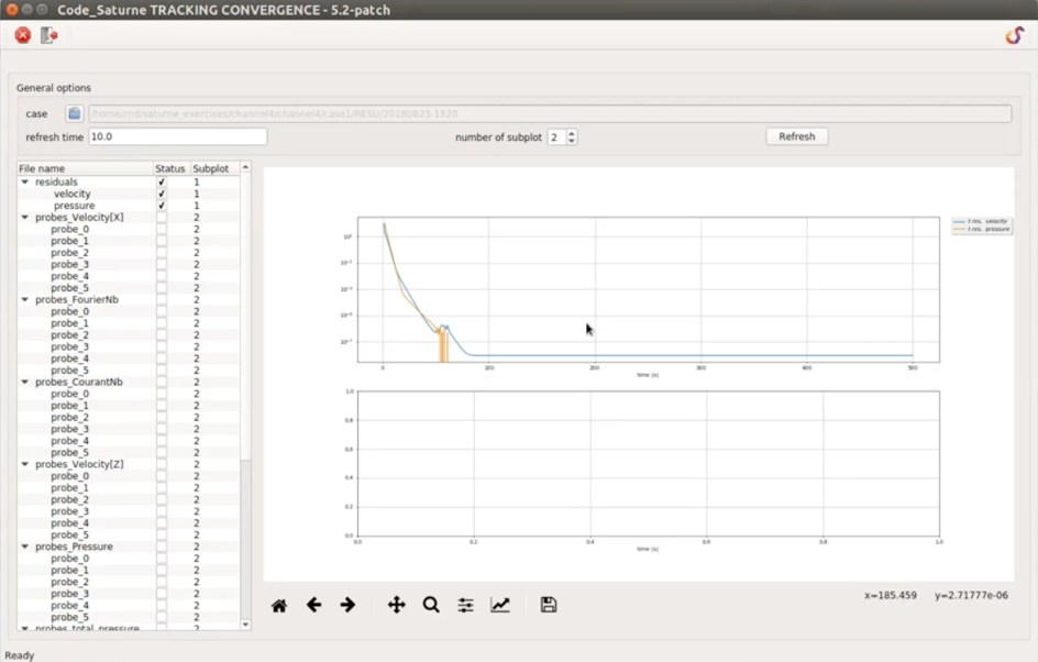
Click on « Convergence tool » to check the convergence status as a graph :

Step 7- Post-processing the data

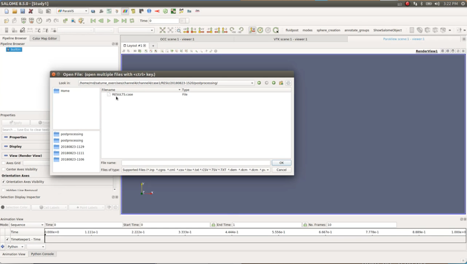
Open the Paravis module and open your data saved into a RESULT.case file

(This file is located in RESU/date of your analysis/post-processing/ folder)

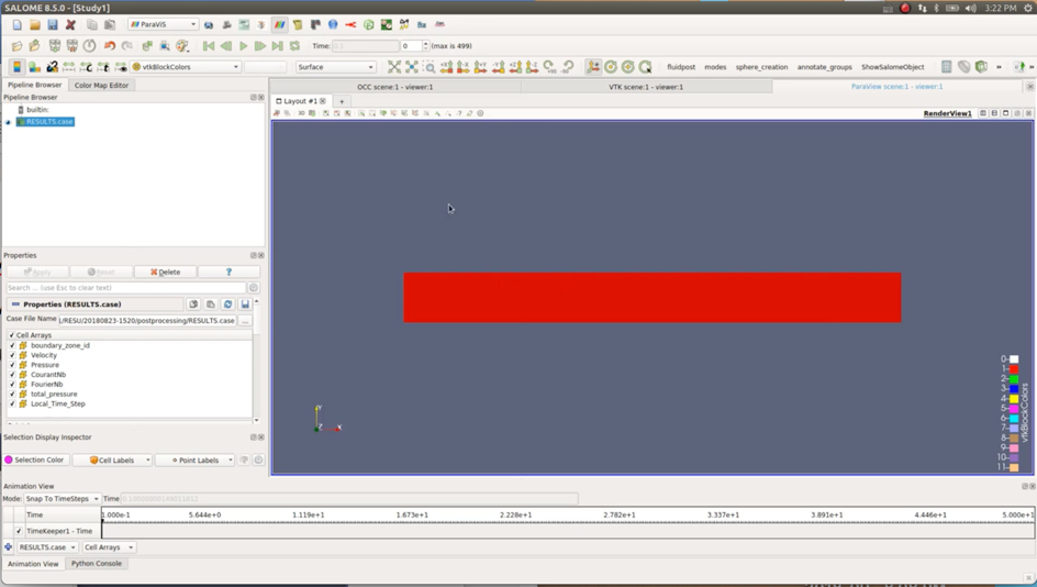
You will get something like that :

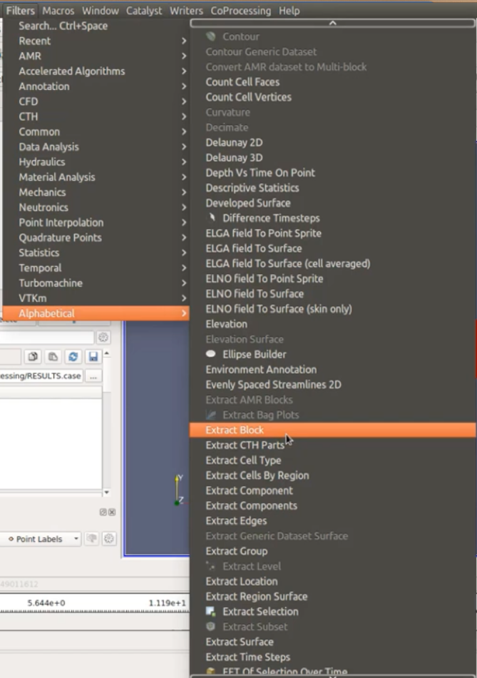
We can’t see directly the results, we have to use the filter « Extract Block » to separate the data from the fluid volume of the rest :

You will then get a visualisation of the pressure and the velocity without node averaging :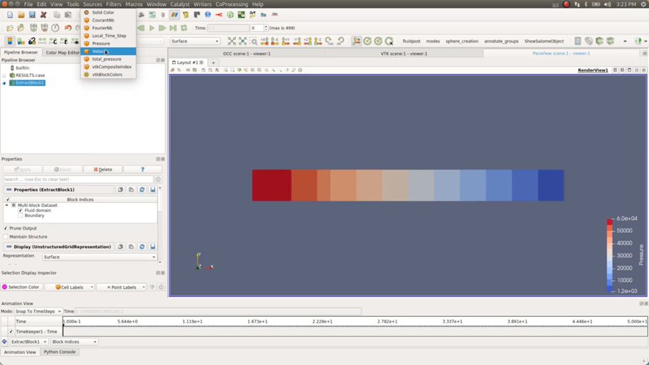

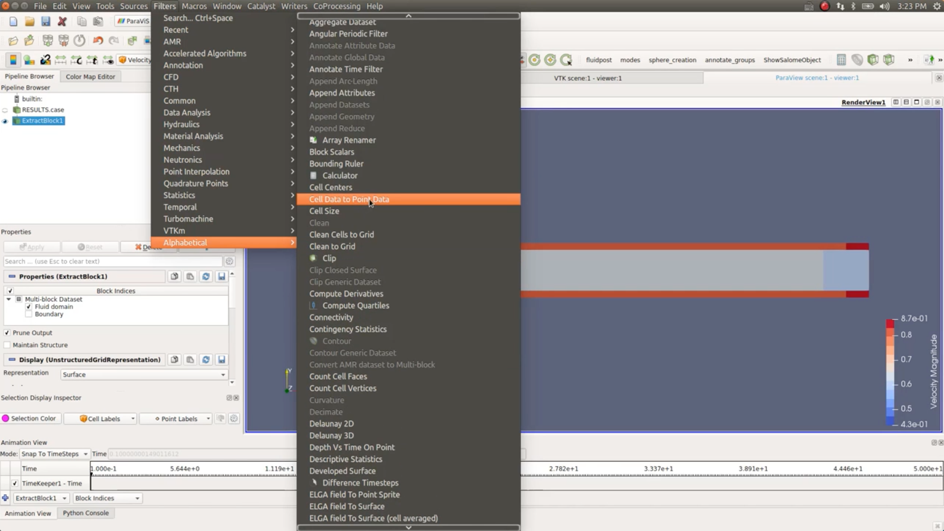
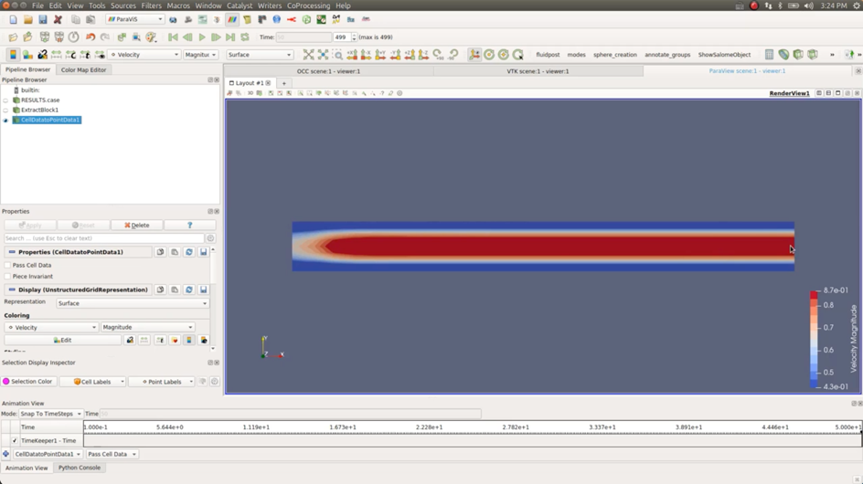
To get this averaging, you need to use the filter « Cell Data to Point Data »

Here’s what you should get for the velocity :

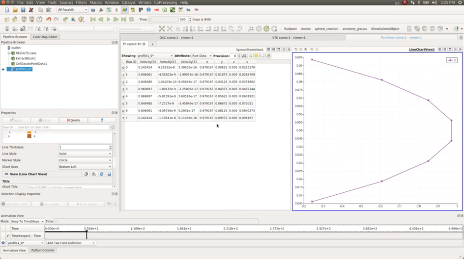
You can finally check the other data like the profile of velocity by opening the file in the same way :

(Watch the video to see the exact way to get this graph in Paravis, that’s a bit tricky if you never used Paravis)

if you want to create this kind of filters (Extract Block/Point Data to Cell Data) in Paravis more easily, you can use macros. Macros can execute the same operations automatically to save time…

If you are interested, maybe I’ll show you how to do that in the next video… let me know if you are interested by leaving a comment!

---

Ok, that’s all for this tutorial of Salome CFD, I hope it was useful and that you learned a lot from it.

If it was, don’t forget to leave a comment and let me know ;-) I’ll make more!

Thanks for following the blog!

–Cyprien “first intro to salomeCFD” Rusu