How to Implement the Lattice Boltzmann Method (LBM) with a single relaxation time collision operator

This article complements and enhance the first article published on the blog about the LBM Method: Everything you need to know about the Lattice Boltzmann Method

Today, the article will focus on the practical implementation of this method! I leave the place now to the author of the article, my friend and engineer Nicolas Maquignon.

After reading the previous article on LBM, some of you wondered how to actually implement or transfer the theoretical knowledge into an effective simulation either for preliminary test cases or applied problems. Today, I am going to provide explanations about how to implement test cases, or even practical simulations. 

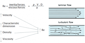
First, I am going to remind you the LB equation (LBE), and we will have a look a the non-dimensionalisation of the LBE, that is a fundamental concept to be familiar with, in the field of LBM. You are going to need to be familiar with this in order to run your simulations in a coherent manner. In the same section, we will have a look at the crucial concept of similarity, using the Reynolds number, which also is an important notion to understand. As for the NS equations, the Reynolds number can be seen as a value that drives the turbulent nature of the flow, but it also can be used to show that two simulations are similar. 

In a second part, I will show you how to implement advises and methods and we are going to talk about which language and environnement are best suited for LB simulations, and I'll even give you some coding tips. I use mylself Linux Ubuntu and C++ language.

We will end the article with some post-processing tips usig Paraview, which is an excellent tool for visualization of results and interpretation.

First, I would like to say that you will only find very rare articles that talk about this topic in a clear sense, as it seems this part is most of time considered obvious by many people that already are in the field of LBM.

A lot of articles on the subject just take adimensionned LB equations without even mentioning it. 

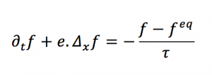
In the first article, we established the following LB equation :

This equation actually is a dimensioned equation, using physical units.

In order to make things more generic, in the field of LBM, we establish an LB equation that is adimensioned. Having generic equations allows you to build a single solver for any kind of fluid. The principle is to define constants that would allow you to recover dimensionned values.

It saves you also time and ressources, and it provides a deep understanding of the meaning of the simulation.

The method is first to define

1. a reference time t0
2. a reference legnth l0
3. a reference density   ρ0
4. and a reference speed   u0 = l0/t0

Then with the use of some algebra the equation becomes :

With some straightforward algebra, it becomes :

With the following expressions, and with the ^ symbol meaning the value is adimensioned:

Though the adimensioned equation is now established, we still need to be more specific on the constraints that have to be taken on the reference values, so that it fits with a space phase space (x,e) mesh.

We could establish those links by recovering Navier-Stokes macroscopic equations using some special technique known as the Chapman-Enskog method. A Chapman-Enskog procedure allows to recover NS equations from the LB equation. Interested readers can refer to scientific articles on the subject (contact me) to have details about the maths we use to to it.

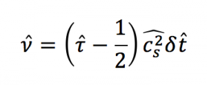
To summarise, such a procedure actually is a decomposition of distribution functions using different time scales. But if we are to skip the maths on the subject, we get a fundamental link among relaxation time, speed of sound and viscosity :

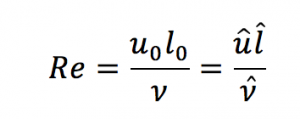
… And as you might already now, viscosity is also used for the Reynolds number:

The two previous relationships are the key for a correct non-dimensionalisation of the LBE.

 Note that the lattice speed of sound (Cs2 has appeared, indeed because the developments that are performed in the Chapman-Enskog expansion use the equilibrium distribution function, that actually contains the speed of sound. These relationships also means that the Reynolds number drives all the caracteristic properties that will be used for the simulation.

This means that for equivalent shaped geometries, boundary conditions and initial conditions, two systems are equivalent as long as they have the same Reynolds number, even though caracteristic length, speed or viscosity are different.

What really matters is the Reynolds number. We could illustrate this property, with the example of the flow past cylinder test case, that I implemented using a D2Q9 (2 space dimensions – 9 discrete velocities) LBM model. For this bechmark, we could for example use the following layout :

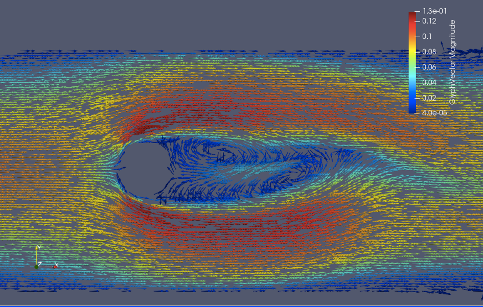
In order to illustrate this section, I found it nice to provide a Paraview illustration of the flow past cylinder simulation with LBM. Here, the Reynolds number is of 2000, and the figure is plotted after some simulation time. We can see the development of two vortex past the cylinder, that would spread if we continue to run the simulation. On the following figure, we observe the velocity vector field, represented in paraview with the glyph filter, from a CSV output obtained with the simulation. In this representation I seeded enough glyph under Paraview, so that we can observe the two vortices past the cylinder, and I used the velocity vector magnitude on jet colormap to show speed magnitude.

To conclude with the dimension problem, here is a list of rules you should use for non-dimensionalisation, in order to be consistent with the Reynods number and similarity. For a fluid with reference density ρ0, reference visocity ν0, and reference sound speed c0, and for a domain discretised with a space step dx, we can use the following properties :

Without any particular mesh refinement, 

If you are interested, you can try to re-demonstrate the previous properties using a Chapman-Enskog procedure. 

After establishing all the theoretical notions, and becoming familiar with what we need to know on LBM, we indeed still need to test our equations with some computer simulation. 

Now... as you probably noticed, it is not sufficient to define only parameters and properties, because even if you really understand what’s going on with the equations, and have a theoretical knowledge of fluid dynamics, it is not of great help if you do not have any programming skills allowing you to translate this knowledge into practical problems solving. 

Furthermore, theoretical knowledge is of almost no interest for a client with a practical problem. What you are expected to do as CFD or FEA engineer is to put your knowledge into practise and bring innovation and solution that would help your company grow or solve your client’s problem. As you know, for many cases you can use commercial softwares, but sometimes they don’t contain enough physics to solve complicated problems.

This means you’re going to need to plugin your physics into the existing software or you can also develop your own computer simulation.

Today, in this article let's explore some computer methods to develop your own simulation using LBM.

First thing to wonder about is the language you want to use to develop your code.

Most of time, people think that scripting language as Matlab are perfect for testing algorithms. It actually is correct, but this only allows to test things on small sized problems, unless you want to spend forever in waiting for your results… Indeed scripting languages are often slow languages unlike compiled languages. But Matlab provides an easy user programming interface and if you’re a newbie to simulation, this might not be a bad idea if you start with such type of language. 

Though scripting languages are easier, I rather advise to use compiled languages as C or C++, because they are designed to be close to computer architecture and they provide a lot of ways to optimize your code. For those interested in multi-threading, you can for example use the openmp library in a very efficient way if you use C/C++. This property is crucial if you want to run simulations in reasonable delays. Multi-threading is of great interest if you run your program on multi-CPU architectures. For example if you use a 6 cores CPU, multi-threading allows you to define a « thread » of execution for each core.

This in some ways means that in a perfect world, your simulation time will decrease by a 6x factor! And imagine the same tool applied on highly parallel architectures as clusters, that can provide you with thousand of CPUs (but of course, not for free!). 

I should also mention about CUDA, which is the most powerful language you could use for your implementation. This language is designed for GPU computing, this means using Graphics Processor Units for scientific computing. A GPU is a coprocessor - it still needs a CPU - that contains thousands of cores. To summarise, a bit like for multi-threading on CPU, a thread is asigned to every cores of the GPU. And as it contains thousands of cores, the speed up factor can be impressive. But the cores of the GPU are not of the same kind of those from the CPU. Every GPU core needs to do the very same operation at the same time, simultaneously. This constraint is to be respected if you want to work your GPU in an efficient manner. On the contrary CPU cores are more independant and are more programmable.

Now that we’ve discussed the possibilities for language of implementation, I propose to have a look in details on the implementation of the advection part of the LBM algorithm. I’ll be using pseudo-C++, and linearized adresses.

(By linearized adresses, I mean that instead of using multidimensional matrixes, I’ll use just one dimensionnal pointers)

 This can be done by translating the adresses that way:

And once again, you might wonder what it means and why the heck should we bother doing such transformations, because as far as today you’ve never seen any reason to complicate your life with such barbarian notations…

First, let’s clarify the meaning of the following function:

if you remember the previous article, it corresponds to the density distribution function at site x with microscopic speed α, at time t. In other words :

Here (i,j,k) symbols are taken for the 3D cartesian geometrical coordinates. Remember that we used x as a 3D space vector, which has 3 coordinates. The notations (i,j,k) are integers that correspond to adimensioned coordinates, as 

X, Y, Z represent the number of elements in the 3 space directions, and Q is the number of discreet speed. Now we need to translate the mathematical formulation into computer language, and in the first place we used C++ multidimension matrix notation

This new notation is a multidimension pointer, it could be used in a C++ program, but most of time it is preferable to use 1D pointer for memory segmention matters. Especially if we are to run simulations with many elements that consume a lot of memory. And more, we should also prefer dynamic memory allocation to static memory allocation. That’s why I translated the 4D pointer to 1D pointer, and this is done that barbarian way :

To explain this, it is as if the rows and columns of your matrix had been concatenated into a single row matrix, and the previous formula gives the way to translate the N-D adress of an element into a single 1-D adress. If you want to convince yourself that it’s correct, try to apply the formula on a small 2D matrix, and you’ll see that it turns your 2D matrix to 1D. Of course, all of this might seem a bit complicated, but what is important to see is that translating maths into effective computer simulation of your own is doable, though it requires some effort…

And the last step of this section, let’s do it for fun, as promised the implementation detail of the advection kernel using C++ pseudo-code. Let us first remind the mathematical formulation of advection in discrete LBE :

We need to translate the left hand side of this equation with linearized adress :

Note that in the C++ version, the time variable has disappeared because time is discrete and a following time step is stocked in the pointer

Using the previous linearized adress and a for loop, so that every element is updated, this translates into :

For those who would like further details, don’t hesitate to contact me.

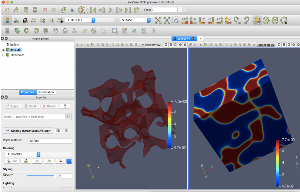
Well, after going through all this fascinating implementation tips, I think it’s time to have a look at the post-processing, because after all, the images you will present to your boss or to your client are the summary of your work, in it’s tangible aspect. I just placed an example of a Paraview post-processing of a 3D LBM simulation of multiphase flow :

In your C++ simulation, you can program a function that writes VTK or CSV files, that you’ll be able to read using Paraview and its filters. Here, on this view, we have a look at the density field of a liquid gaz system that is undergoing a condensation process. On the very left, you can see that the file data.vtk is opened. You can easily create a vtk file from you’re C++ simulation. Then, as an example, I plotted on right the density field using some surface type representation. Surface is on the options of the top tool bar, as you can see on the picture. On left, I applied a threshold so that only liquid density is represented. You can see the use of the threshold filter in the pipeline of filters on the very left. And this gives quite a cool view about what’s going on in a condensation process!!

———–

That’s all basically for this article… and that's a LOT of knowledge to unpack ;-)

Take all the time you need to read and if you want to share your ideas, please just write what you think in the comments and let me know

Thank you so much for reading, I hope you learned a lot!

–Cyprien